HW 6:
How to clone your repo
You clone your homework-5 repo exactly how we have been cloning AEs! Please see Moodle for more information.
How to turn your HW in
Homework is turned in via Gradescope. You can find the Gradescope HW-5 button on our Moodle page. Please remember to select your pages correctly when turning in your assignment. For more information, please see on Moodle: Submit Homework on the Gradescope Website.
How to format your Homework
For each question (ex. Question 1), put a level two (two pound signs) section header with the name of the question.
For questions with multiple parts (ex. a, b, c), please put these labels in bold as normal text.
For example…
Question 1
a
This homework is due Sunday, November 16th at 11:59pm.
You will need to have at least 3 (meaningful) commits by the end of your homework assignment. Please practice proper version control techniques by committing and pushing after each answered question.
Packages
Start your document by making a Packages header, and copying this code and code chunk over into your .qmd file.
Use message: false and warning: false as code chunk arguments for this code chunk so you don’t get all of the extra unnecessary information when you render your document.
Question 1: Reading in your own data
We have spend a lot of time working with pre-packaged data in this course. I want to make sure you leave with an understanding on how to upload and work with your own data. We are going to work through some examples from the following reading in our textbook:
Note: I DO NOT want you to read in the data using the following code: students <- read_csv("https://pos.it/r4ds-students-csv")
The purpose of this assignment is to be able to take a csv, put it into a data folder, and read in your data using a correct file path.
a Download the student.csv data set from Moodle onto your computer. Next, upload your data into the data folder on your posit container. Lastly, use the following code to read in your data..
students <- read_csv("data/students.csv")**take a glimpse of your students object to show that you have uploaded the data correctly.
glimpse(students)Rows: 6
Columns: 5
$ `Student ID` <dbl> 1, 2, 3, 4, 5, 6
$ `Full Name` <chr> "Sunil Huffmann", "Barclay Lynn", "Jayendra Lyne", "Leo…
$ favourite.food <chr> "Strawberry yoghurt", "French fries", "N/A", "Anchovies…
$ mealPlan <chr> "Lunch only", "Lunch only", "Breakfast and lunch", "Lun…
$ AGE <chr> "4", "5", "7", NA, "five", "6"b Pipe your students object into the following janitor::clean_names().
For this question, answer the following…
– What is the :: doing in-between janitor and clean_names()
– What is the clean_names() function doing?
Hint: Take a look at this stack exchange forum here or look at the 10.7 Summary in our book here and click the ↩︎!
students |>
  janitor::clean_names()
# A tibble: 6 × 5
student_id full_name favourite_food meal_plan age
<dbl> <chr> <chr> <chr> <chr>
1 1 Sunil Huffmann Strawberry yoghurt Lunch only 4
2 2 Barclay Lynn French fries Lunch only 5
3 3 Jayendra Lyne N/A Breakfast and lunch 7
4 4 Leon Rossini Anchovies Lunch only <NA>
5 5 Chidiegwu Dunkel Pizza Breakfast and lunch five
6 6 Güvenç Attila Ice cream Lunch only 6 the :: calls the function (on the left) from the exact package (on the right). This is useful, in that different functions can have the same name / you don’t need to library the package to explicitly call for it.
clean_names() makes all letters lower case + removes spaces.
c Save your pipeline in part b named clean_data.
clean_data <- students |>
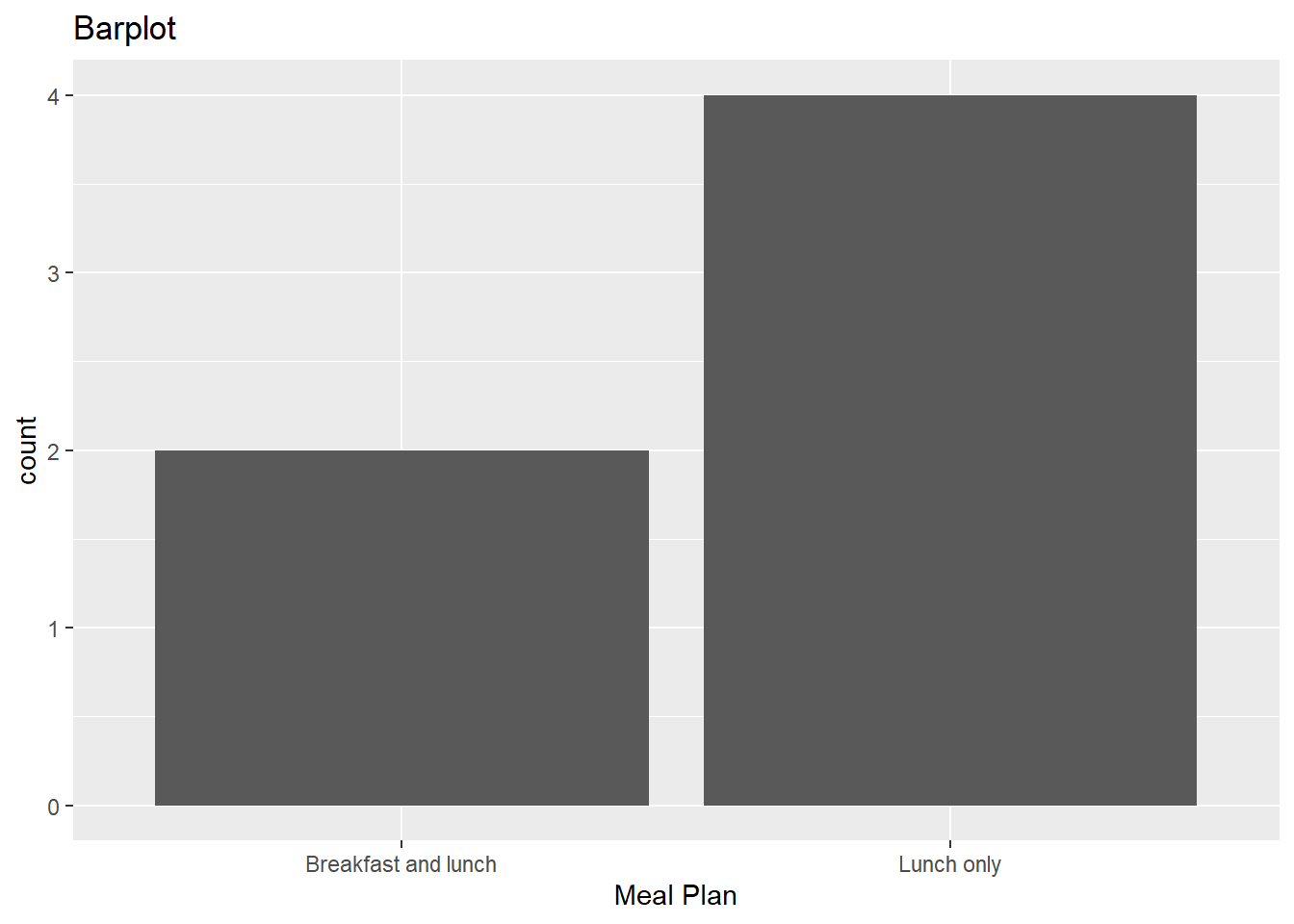
janitor::clean_names()d Now, use your new named R object from part c to make a barplot with mealPlan on the x axis. Add appropriate labels
Question 2: Admissions
For this question, we are going to investigate the relationship between if someone was admitted to graduate school admit, with explanatory variables gre and gpa. Please read in the data using the following code below.
gpa - grade point average
gre - graduate record examinations score
admit - 1 if you were accepted; 0 if you were not accepted
a Make a summary table that shows the mean gre and mean gpa for each level of the admit variable.
# A tibble: 2 × 3
  admit   gre   gpa
  <fct> <dbl> <dbl>
1 0      573.  3.34
2 1      619.  3.49
b Now, fit your generalized linear additive model below. That is, fit an additive model where gre and gpa are both of your explanatory variables. Hint: just like in linear regression, we can do this using +.
Call:
glm(formula = admit ~ gre + gpa, family = "binomial", data = mydata)

Coefficients:
             Estimate Std. Error z value Pr(>|z|)
(Intercept) -4.949378   1.075093  -4.604 4.15e-06 ***
gre          0.002691   0.001057   2.544   0.0109 *
gpa          0.754687   0.319586   2.361   0.0182 *
---
Signif. codes:  0 '***' 0.001 '**' 0.01 '*' 0.05 '.' 0.1 ' ' 1

(Dispersion parameter for binomial family taken to be 1)

    Null deviance: 499.98  on 399  degrees of freedom
Residual deviance: 480.34  on 397  degrees of freedom
AIC: 486.34

Number of Fisher Scoring iterations: 4
c Write out your estimated model to model the probability of getting into graduate school. You can get the estimates of your model by running summary() on your response.
$$
=
$$
d Using your model, make a prediction on the probability of being administered to graduate school. Include se.fit = TRUE in the predict argument to compute the standard error associated with this prediction. We are going to use this value in part e.
predict(model1, data.frame(gre = 620, gpa = 2.89), type = "response", se.fit = TRUE)$fit
1
0.2497194
$se.fit
1
0.04005892
$residual.scale
[1] 1e Using a critical value of 1.96, calculate a prediction interval that estimates the true probability of getting into graduate school for someone with a gpa of 2.89 and gre score of 620.
0.250 + 0.04*1.96[1] 0.32840.250 - 0.04*1.96[1] 0.1716The 95% prediction interval is (0.172, 0.328).
f Based on your answer to part e, give this individual a recommendation on if they should apply to graduate school, justify your answer.
The 95% prediction interval is entirely below .5. Because of this, I would not recommend someone with a gre score of 620 and a gpa of 2.89 to apply to graduate school.
g You just created your first prediction interval above! This is slightly different than a confidence interval. Read the following article here up through Confidence Interval vs Prediction Interval: A Summary. Next, answer the following question(s)
answers will vary
– describe one similarity between a confidence interval and a prediction interval
they are centered at the same value!
– describe one difference between a confidence interval and a prediction interval
prediction intervals are always wider!
Submission
- Go to http://www.gradescope.com and click Log in in the top right corner.
- Log in with your school credentials.
- Click on your STA 511 course.
- Click on the assignment, and you’ll be prompted to submit it.
- Mark all the pages associated with exercise. All the pages of your homework should be associated with at least one question (i.e., should be “checked”). If you do not do this, you will be subject to lose points on the assignment.
- Do not select any pages of your PDF submission to be associated with the “Workflow & formatting” question.
The “Workflow & formatting” grade is to assess the reproducible workflow. This includes:
- linking all pages appropriately on Gradescope
- putting your name in the YAML at the top of the document
- Pipes
%>%,|>and ggplot layers+should be followed by a new line - Number of GitHub committs.
- You should be consistent with stylistic choices, e.g.
%>%vs|>
Grading for HW-6
- Exercise 1: 15 points
- Exercise 2: 30 points
- Workflow + formatting: 5 points
- Total: 50 points