HW 5: Regression + Chi-Square
How to clone your repo
You clone your homework-5 repo exactly how we have been cloning AEs! Please see Moodle for more information.
How to turn your HW in
Homework is turned in via Gradescope. You can find the Gradescope HW-5 button on our Moodle page. Please remember to select your pages correctly when turning in your assignment. For more information, please see on Moodle: Submit Homework on the Gradescope Website.
How to format your Homework
For each question (ex. Question 1), put a level two (two pound signs) section header with the name of the question.
For questions with multiple parts (ex. a, b, c), please put these labels in bold as normal text.
For example…
Question 1
a
This homework is due Sunday, November 16th at 11:59pm.
You will need to have at least 3 (meaningful) commits by the end of your homework assignment. Please practice proper version control techniques by committing and pushing after each answered question.
Packages
Start your document by making a Packages header, and copying this code and code chunk over into your .qmd file.
Use message: false and warning: false as code chunk arguments for this code chunk so you don’t get all of the extra unnecessary information when you render your document.
Note: There are multiple choice questions in this assignment. Please make sure to copy the sentence over into your quarto document.
Data
For this homework, we are going to being using the survey data set from the MASS package. This data frame contains the responses of 237 Statistics I students at the University of Adelaide to a number of questions. You can find the variable names and descriptions by pulling up the help file for survey.
We are going to use a cleaned up data set that only looks at students younger than 25 years old. Include this piece of code in your document before you start your exercises. There will be 153 total observations after running this code.
Exercise 1
In this exercise, we are going to investigate the relationship between a student’s age and their Pulse. Please pull up the help file for survey using ?suvey in the Console (after running your packages) to learn more about the variables. For this question, use Pulse as our response variable, and Age as our explanatory variable.
Justify, in as much detail as possible, why we can’t use difference in means methodology to analyze these data.
Using
summarise()andcor(), calculate the correlation coefficient betweenPulseandAge.
- Write out the appropriate interpretation of your correlation coefficient in part b by selecting the most appropriate interpreation below.
– There is a strong positive linear relationship between Age and Pulse.
– There is a weak positive linear relationship between Age and Pulse.
– There is a strong negative linear relationship between Age and Pulse.
– There is a weak negative lienar relationsihp between Age and Pulse.
– There is a strong negative relationship between Age and Pulse.
– There is a weak negative relationship between Age and Pulse.
- Create a scatterplot (with appropriate labels), and fit a linear line of best fit through these data using
geom_smooth(). You can turn the SE band off by setting SE = F as an argument withingeom_smooth(). Be mindful to put your response variable on the y-axis, and include appropriate labels.
- Copying the code below, fit a simple linear regression model that will provde you the coefficients of the line you fit in part d. In a separate line of code in the same R chunk, produce your output using
tidy(model1).
model1 <- lm(Pulse ~ Age, data = survey)Interpret your slope coefficient in the context of the problem.
Interpret your intercept in the context of the problem.
Exercise 2: Hypothesis Test
We are now going to conduct a hypothesis test to test for a linear relationship between Pulse and Age.
- Write out your appropriate null and alternative hypotheses in proper notation below. Note: You do not have to use LaTeX. You may simply spell out the notation.
\(Ho:\)
\(Ha:\)
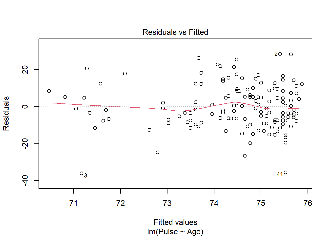
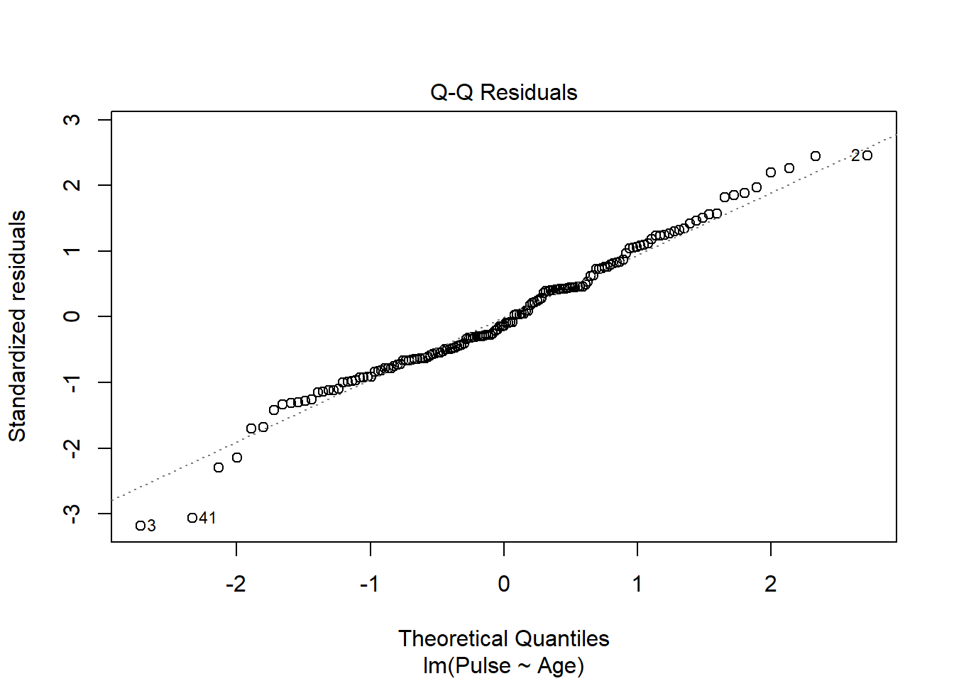
- You may assume that one student is independent of the other. See the following plots below. You may or may not include this code in your document.
Use the plots to discuss the following assumptions in 1-2 sentences each:
– Linearity
– Equal Variance
– Normality
- Using your model output, what type of statistic is -1.32?
– F
– \(\chi^2\)
– t
– z
Using your model output, show how -1.32 was calculated.
Using an \(\alpha\) value of 0.05, select the appropriate decision and conclusion.
– With a p-value larger that 0.05, we fail to reject the null hypothesis, and have weak evidence to conclude a true linear relationship between a student’s Age and Pulse.
– With a p-value larger that 0.05, we reject the null hypothesis, and have weak evidence to conclude a true linear relationship between a student’s Age and Pulse.
– With a p-value smaller that 0.05, we fail to reject the null hypothesis, and have weak evidence to conclude a true linear relationship between a student’s Age and Pulse.
– With a p-value smaller that 0.05, reject the null hypothesis, and have strong evidence to conclude a true linear relationship between a student’s Age and Pulse.
Exercise 3
In this exercise, we are again going to also the survey data set. We are going to test if a student’s smoking status in independent from how often they exercise. As a reminder, you can find the variable names and descriptions by pulling up the help file for survey.
- Make an observed table (tibble output) using
group_by()andsummarise()that counts the frequency of every exercise by smoking combination. Your answer should be a 11 x 3 tibble. Add to the existing pipeline that filters out missing values for smoking when reporting your tibble.
- Below is a table of expected counts. These are counts that would expect to see if exercise really has no impact on smoking status.
           survey$Smoke
survey$Exer     Heavy     Never     Occas     Regul
       Freq 3.0196078 61.901961 6.0392157 6.0392157
       None 0.4705882  9.647059 0.9411765 0.9411765
       Some 2.5098039 51.450980 5.0196078 5.0196078
Question: Using the values from a, recreate the expected count of those who smoke heavy and exercise frequently. Show your work.
Are you justified to use theory based procedures to carry out a chi-square test of independence? Justify your answer
Regardless of your answer, the results from a chi-square test of independence can be seen below…
    Pearson's Chi-squared test

data:  survey$Exer and survey$Smoke
X-squared = 1.4117, df = 6, p-value = 0.9651Question: Please explain how df = 6 was calculated when carrying out this test.
- Using the results from the output in part d, report the test statistic, p-value, and distribution the p-value was calculated from. Be specific.
You do not need to write a decision, conclusion, or anything other than what the question is asking.
Submission
- Go to http://www.gradescope.com and click Log in in the top right corner.
- Log in with your school credentials.
- Click on your STA 511 course.
- Click on the assignment, and you’ll be prompted to submit it.
- Mark all the pages associated with exercise. All the pages of your homework should be associated with at least one question (i.e., should be “checked”). If you do not do this, you will be subject to lose points on the assignment.
- Do not select any pages of your PDF submission to be associated with the “Workflow & formatting” question.
The “Workflow & formatting” grade is to assess the reproducible workflow. This includes:
- linking all pages appropriately on Gradescope
- putting your name in the YAML at the top of the document
- Pipes
%>%,|>and ggplot layers+should be followed by a new line - Number of GitHub committs.
- You should be consistent with stylistic choices, e.g.
%>%vs|>
Grading for HW-5
- Exercise 1: 15 points
- Exercise 2: 20 points
- Exercise 3: 15 points
- Workflow + formatting: 5 points
- Total: 55 points