Homework-3
How to clone your repo
You clone your homework-3 repo exactly how we have been cloning AEs! Please see Moodle for more information.
How to turn your HW in
Homework is turned in via Gradescope. You can find the Gradescope HW-3 button on our Moodle page. Please remember to select your pages correctly when turning in your assignment. For more information, please see on Moodle: Submit Homework on the Gradescope Website.
How to format your Homework
For each question (ex. Question 1), put a level two (two pound signs) section header with the name of the question.
For questions with multiple parts (ex. a, b, c), please put these labels in bold as normal text.
For example…
Question 1
a
This homework is due Sunday, October 5th at 11:59pm.
You will need to have at least 3 (meaningful) commits by the end of your homework assignment. Please practice proper version control techniques by committing and pushing after each answered question.
Packages
Start your document by making a Packages header, and copying this code and code chunk over into your .qmd file.
Use message: false and warning: false as code chunk arguments for this code chunk so you don’t get all of the extra unnecessary information when you render your document.
Exercise 1 (15 points)
For each scenario, write out the appropriate null and alternative hypothesis in proper notation.
- A professor wants to know if the average exam score for her class is different from the historical average of 80 on a standardized test. She believes her class will perform differently due to a new teaching method.
\(H_o: \mu = 80\)
\(H_a: \mu \neq 80\)
- A space agency wants to compare the reliability of two different private companies, Provider A and Provider B, for launching satellites into orbit. The agency collects data on their recent launch history. Provider A has completed 200 launches, with 192 of them being successful. Provider B has completed 150 launches, with 138 of them being successful. The space agency wants to investigate if Provider B has less safe launches, as they tend to user older technologies.
\(H_o: \pi_a - \pi_b = 0\)
\(H_a: \pi_a - \pi_b > 0\)
- A politician claims that they have an approval rating of at least 50%. A political analyst wants to test this claim and believes the true approval rating is lower.
\(H_o: \pi = .5\): it is acceptable to use \(\geq\)
\(H_a: \pi < .5\)
Exercise 2
Exploratory data analysis: Murderous Nurse (20 points)
For several years in the 1990s, Kristen Gilbert worked as a nurse in the intensive care unit (ICU) of the Veterans Administration Hospital in Northampton, Massachusetts. Over the course of her time there, other nurses came to suspect that she was killing patients by injecting them with the heart stimulant epinephrine. Gilbert was eventually arrested and charged with these murders. Part of the evidence presented against Gilbert at her murder trial was a statistical analysis of 1,641 randomly selected eight-hour shifts during the time Gilbert worked in the ICU. For each of these shifts, researchers recorded two variables: whether Gilbert worked on the shift and whether at least one patient died during the shift.
The data set you will be working with is called gilbert. Run the code below to create the data set.
- What are the observational units. That is, whom or what exactly are the data being collected off of.
The shifts
- Classify each variable as categorical or quantitative. Additionally, classify if this is our response variable or explanatory variable.
Whether Gilbert worked on the shift categorical explanatory
Whether at least one patient died during the shift categorical response
- Create a summary table using
summarize()andgroup_by()to summarize these data. Next write out your statistic in proper notation.
`summarise()` has grouped output by 'outcome'. You can override using the
`.groups` argument.
# A tibble: 4 × 3
# Groups: outcome [2]
outcome working count
<chr> <chr> <int>
1 died gilbert 40
2 died no-gilbert 34
3 no-death gilbert 217
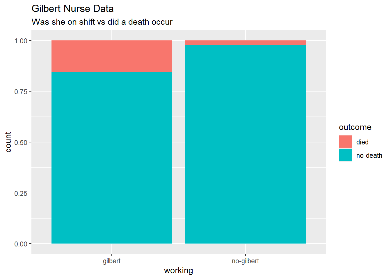
4 no-death no-gilbert 1350- Now, create a proper data visualization to help explore these data. Comment on a patterns you observe with these data. Hint: In the appropriate
geom, useposition = "fillto create a visualization that is easier to read when we have differing sample sizes. Include appropriate labels.
Inference: Murderous Nurse (Confidence Interval) (40 points)
Before we explore Kristen Gilbert, we want to investigate the proportion of deaths at this hospital, by itself. Specifically we want to estimate the true proportion of deaths at this hospital.
- Report the appropriate statistic, using proper notation, for the proportion of deaths at this hospital, regardless if Gilbert was working.
\(\hat{p} = \frac{74}{1641}\)
- Can we justify creating a 90% confidence interval? That is, can we trust the results? Justify your answer below.
Yes. The context of the probelm claims that these shifts were take from a random sample of all shifts Gilbert worked. Therfore, we can assume that one shift does not influence the shift of another. Additionally, we don’t have evidence to reject the normality assumption.
0.045 * 1641 ~ 73 > 10
(1 - 0.045) * 1641 ~ 1567 > 10
- Regardless to your answer in part b, we are going to create a 90% confidence interval. First, use
qnorm()to find the appropriate \(Z^*\) to create a 90% confidence interval.
- Now, calculate the SE(\(\hat{p}\)). Show your work.
\[SE_{\hat{p}} = \sqrt{\frac{\left(\frac{74}{1641}\right)\left(1 - \frac{74}{1641}\right)}{1641}} = 0.00512\]
- Report your margin of error here.
\(ME = SE(\hat{p}) * z^*\) = 0.0084
- Now report your 90% confidence interval AND interpret it in the context of the problem.
\(0.045 \pm 0.0084 = (0.0366, 0.0534)\)
We are 90% confident that the true proportion of deaths observed on shifts at the hospital is between 0.0366 and 0.0534.
- Now, calculate a 70% confidence interval. Use
qnorm()to find the appropriate \(Z^*\). You do not have to interpret this confidence interval.
qnorm(.85, 0, 1 , lower.tail = TRUE)[1] 1.036433\(0.045 \pm 1.036 * 0.00512 = (0.03970, 0.05030)\)
- Discuss one benefit and one drawback of having a lower confidence level below.
Benefit: A lower confidence interval is more narrow / precise.
Drawback: In the long run, we would expect our confidence intervals to capture the true population parameter of interest less often.
- Interpret your confidence level (90%) below. That is, what is the meaning of 90% confident? Note: This is not an interpretation of your single confidence interval.
If we make many many 90% confidence intervals under similar conditions, we would expect roughly 90% of all confidence intervals made to actually capture the true population parameter of interest.
Inference: Murderous Nurse (Hypothesis Test) (20 points)
Now, we are going to investigate if there is a relationship between Gilbert working, and deaths at the hospital. Specifically, we want to investigate if there more deaths occur while Gilbert is working.
- Write out your null and alternative hypotheses below in both words and in proper notation. Use informative subscripts.
Ho: \(\pi_w - \pi_n = 0\)
Ha: \(\pi_w - \pi_n > 0\)
where w = working and n = not working
Ho: The true proportion of shifts that observed a death while Gilbert was working is the same as when she was not working.
Ha: The true proportion of shifts that observed a death while Gilbert was working is different than when she was not working.
- We are now going to conduct a Z-test to test your null/alternative hypothesis.
Before conducting this test, justify if we can trust the results of a z-test below? Why or why not.
We can still assume independence, as the sampling scheme was a random sample. This helps us justify that the shifts when gilbert was working on independent of each other, the shifts Gilbert was not working are independent from each other, and the shifts are independent across groups.
We also can check the normality assumption as so:
\(p_\text{pooled} = {74}{1641} = 0.045\)
0.045 * 257 = 11.57 > 10
(1 - 0.045) * 257 = 245.44 > 10
0.045 * 1384 = 62.28 > 10
(1 - 0.045) * 1384 = 1321.72 > 10
- Regardless of your answer, calculate your z-statistic below. Show your work.
\[Z = \frac{\left(\frac{40}{257} - \frac{34}{1384}\right) - 0}{\sqrt{\frac{74}{1641}\left(1 - \frac{74}{1641}\right)\left(\frac{1}{257} + \frac{1}{1384}\right)}} = 9.291\]
- Use the
pnorm()function to calculate a p-value for this hypothesis test.
pnorm(9.291 , 0 , 1, lower.tail = FALSE)[1] 7.642273e-21- Now, write an appropriate decision and conclusion in the context of the problem.
With a p-value of < 0.001, we reject the null hypothesis, and have strong evidence to conclude that the true proportion of at least one death observed on shifts when Gilbert was working is larger than when she wasn’t working.
Exercise 3 (10-points)
A software company wants to test if a new user interface (UI) design for its mobile app affects the proportion of users who complete a core task (e.g., sharing a photo). They set up an A/B test with a control group (Old UI) and a test group (New UI). They set up the following hypotheses:
\(H_o: \pi_n - \pi_o = 0\)
\(H_a: \pi_n - \pi_0 \neq 0\)
After they collect some data, they calculate a z-statistic of -0.34, with an estimated p-value of 0.734.
The researchers than conclude that there is no difference between the true proportion of users in the test group who complete a core task vs the true proportion of users in the control group who complete a core task.
In ask much detail as possible, critique and correct their claim.
Answer: You can not conclude the null hypothesis to be true. We are specific with our language reject or fail to reject. It’s very similar to guilty or not guilty. We do not proclaim someone innocent.
In hypothesis testing, we can not claim the null to be true because, under identical circumstances, we could have very large p-values for multiple different null values. Which one is true? Well… we don’t know… and a hypothesis test does not set out to set a single value to a population parameter.