Exam 1 - Take-home

Solutions

By submitting this exam, I hereby state that I have not communicated with or gained information in any way from my classmates during this exam, and that all work is my own.

Any potential violation of the NC State policy on academic integrity will be reported to the Office of Student Conduct & Community Standards. All work on this exam must be your own.

1. This exam is due Friday, October 17th, at 11:59PM. Late work is not accepted for the take-home.
2. You are allowed to ask content clarification questions via email. Any question(s) that give you an advantage to answering a question will not be answered.
3. This is an individual exam. You may not use your classmates or AI to help you answer the following questions. You may use all other class resources.
4. Show your work. This includes any and all code used to answer each question. Partial credit can not be earned without any work shown.
5. Round all answers to 3 digits (ex. 2.34245 = 2.342)
6. Only use the functions we have learned in class unless the question otherwise specifies. If you have a question about if a function is allowed, please send me an email.
7. If you are having trouble recreating a plot exactly, you still may earn partial credit if you recreate the plot partially.
8. You must have at least 3 meaningful commits on your exam1 repo. If you do not, you will lose Workflow and Formatting points.

Do not forget to render after each question! You do not want to have rendering issues close to the due date.

Reminder: Unless you are recreating a plot exactly, all plots should have appropriate labels and not have any redundant information.

Reminder: The phrase “In a single pipeline” means not stopping / having no breaks in your code. An example of a single pipeline is:

penguins |> 
  filter(species == "Gentoo") |>
  summarize(center = mean(bill_length_mm))

A break in your pipeline would look like:

Gentoo_data <- penguins |> 
  filter(species == "Gentoo")
  
Gentoo_data |>
  summarize(center = mean(bill_length_mm))

Reminder: LaTex is not required for the exam.

Reminder: Use help files! You can access help files for functions by typing ?function.name into your Console.

Good luck!

How to turn your exam

The exam is turned in exactly how you have been turning in homework, via Gradescope. You can find the Gradescope exam1 button on our Moodle page, or go to gradescope.com. Please remember to select your pages correctly when turning in your assignment. For more information, please see on Moodle: Submit Homework on the Gradescope Website.

How to format your Exam

You are asked to format your exam exactly how you would format your homework assignment.

For each question (ex. Question 1), put a level two (two pound signs) section header with the name of the question.

For questions with multiple parts (ex. a, b, c), please put these labels in bold as normal text.

For example…

Question 1

a

Exam Start

Packages

You will need the following packages for the exam.

library(tidyverse)
library(tidymodels)
library(palmerpenguins)
library(dplyr)
library(scales)

Now is a good time to save, render, and commit/push your changes to GitHub

Question 1: Package questions

1. When you render your exam (also see above), you will notice a lot of additional warnings and messages underneath the library(tidyverse), library(tidymodels) and library(palmerpenguins) code.

-- Warning...

-- Attaching core tidyverse packages ...

-- Conflicts ...

etc...

Solution: You can turn messages off using code chunk options with #| message: false and #| warning: false

Hide the all the unnecessary text (not the code itself) using the appropriate code chunk argument for the packages code chunk. You do not need to include any text to answer this question (just hide all the extra text). Hint: You can find a list of these arguments here in the Options available for customizing output include: towards the top.

2. Describe, in detail, the difference between the library() function, and the install.packages() function.

Solution: install.packages() downloads the R-package from CRAN onto your local computer. You only need to do this once. library() “opens up” your package so you can use all of the “tools” inside the package. This needs to be done every time you open your session.

3. Suppose someone you know forgets to library their packages, and instead just try to run the following code.

penguins |>
  summarize(mean_peng = mean(bill_length_mm)

What will the code exactly produce? Why?

Solution: Without running library() on your packages, R would not know what the R object penguins is, summarize() is, etc. These are functions/data in other packages not default in base-R.

You may also have commented on the missing ) for full credit.

Now is a good time to save, render, and commit/push your changes to GitHub

Question 2: Flights Hypothesis Test

Data

Read in the airplanes_data.csv using the code below.

Please copy this code an include it in your assignment to read in the data for this question.

airplanes <- read_csv("https://st511-01.github.io/data/airplanes_data.csv")

For question 2, we will be using the following variables:

flight_distance - distance in miles

customer_type - categorized as either Disloyal Customer or Loyal Customer

A disloyal customer is a customer who stops flying from the airline. A loyal customer is someone who continues flying with the airline. You are specifically interested in miles traveled, and if this varies by customer type.

Use the order of subtraction loyal - disloyal. These data are a random sample of all flights from the year 2007.

For this question, you are asked to conduct a hypothesis test to see if there is a difference between the mean distance in miles traveled for different types of customers.

1. Label your variables as either explanatory/response, and categorical/quantitative, below.

solution: flight_distance is our quantitative response variable; customer_type is our categorical explanatory variable

2. Report your sample mean for each group (using R code) below. Then, write out exactly what your sample statistic is in proper notation.

solution

airplanes |>
  group_by(customer_type) |>
  summarize(mean = mean(flight_distance),
            sd = sd(flight_distance), 
            n = n())

# A tibble: 2 × 4
  customer_type      mean    sd     n
  <chr>             <dbl> <dbl> <int>
1 disloyal_customer 1925.  522.    86
2 loyal_customer    1892.  990.   406

\(\bar{x_l}\) = 1892

\(\bar{x_d}\) = 1925

\(\bar{x_l} - \bar{x_d}\) = ~ -33

3. Write our your null and alternative hypothesis in proper notation.

\(H_o: \mu_l - \mu_d = 0\)

\(H_o: \mu_l - \mu_d \neq 0\)

4. Can we justify conducting a t test? Show your work below.

solution

In order to conduct a t-test, we need to check two assumptions:

– Independence

– Normality

In order to assess independence, we need to look at the sampling scheme. Because the context of the problem suggests that these flights are a random sample from a larger population of flights, we can assume that one flight is independent from another flight.

In order to assess normality, we need to check our sample size, and look for extreme skew/outliers. Based on the output above, we have n = 86 and n = 406. Further, we can see the following data to check for skew/outliers.

airplanes |>
  ggplot(
    aes(x = customer_type, y = flight_distance)
  ) +
  geom_boxplot() + 
  labs(x = "customer type",
       y = "flight distance",
       title = "Boxplot")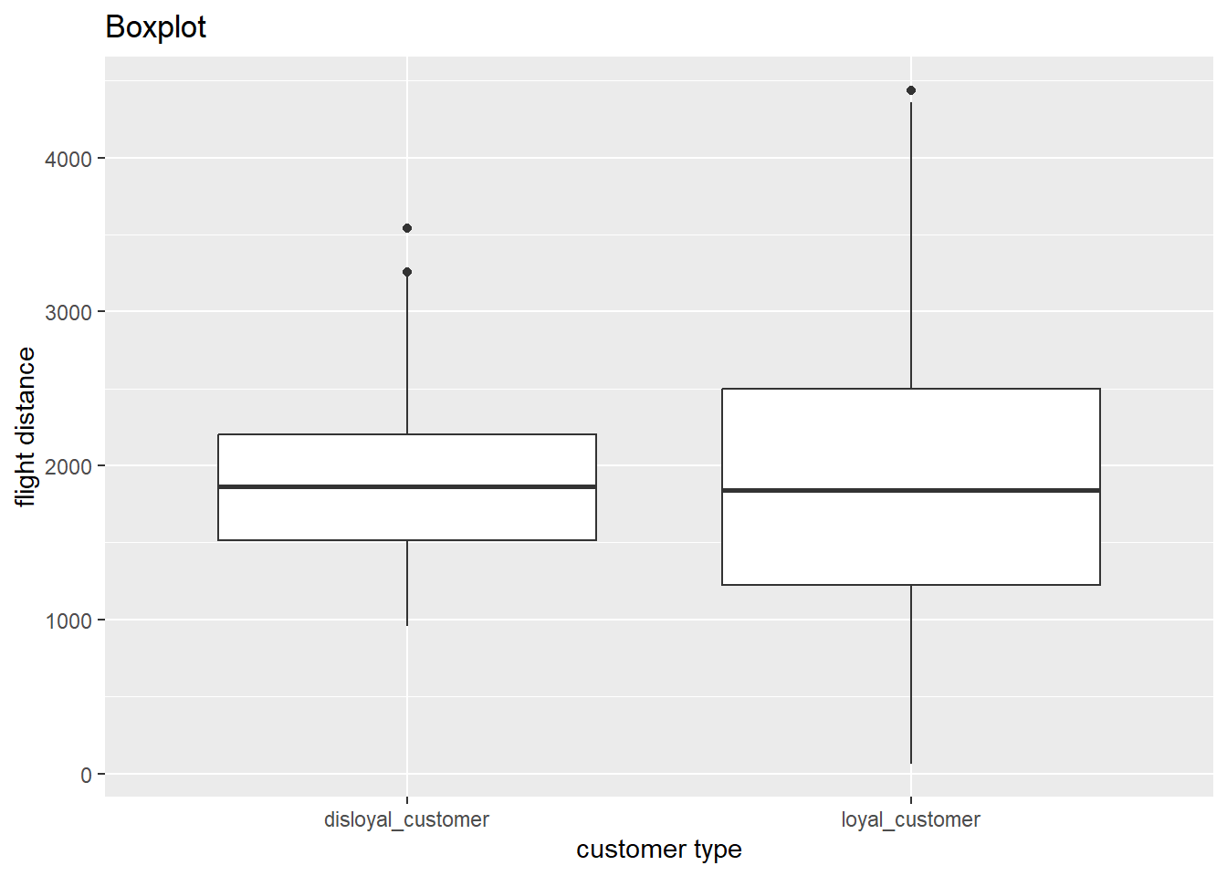

Based on our data visualization, we don’t see any significant skew/outliers, and our large sample sizes, we don’t have enough evidence that the assumption of normality is violated.

5. Regardless of your answer to part d, we are going to conduct a t-test to test your null and alternative hypotheses in part c. First, calculate your t-statistic below. Show your work.

solution

The formula for our t-statistic is as follows:

\(t = \frac{(\bar{x}_1 - \bar{x}_2)}{\sqrt{\frac{s_1^2}{n_1} + \frac{s_2^2}{n_2}}}\)

Thus, our t-statistic is roughly:

\(SE(\bar{x_l} - \bar{x_d}) = \sqrt{\frac{522.0^2}{86} + \frac{990.0^2}{406}} = \sqrt{3168.08 + 2410.34} = \sqrt{5578.42} \approx 74.72\)

\(t = \frac{- 33.0}{74.72} \approx - 0.442\)

6. Use the appropriate R function to calculate your p-value.

solutions The conservative estimate for degrees of freedom we have learned in class is min(n1 - 1, n2 - 1).

min(86 - 1, 406 - 1) = 85.

So, we can calculate our p-value:

pt(-0.442, df = 85, lower.tail = TRUE) * 2

[1] 0.6596117

Because our test is two-sided, we need to look both to the left of our statistic, and to the right of the absolute value of our statistic. This means it’s critical to specify lower.tail = T (if you put in a negative statistic). We can multiply our p-value by 2 because we know our t-distribution is symmetric.

7. Interpret your p-value in the context of the problem. This is different than writing a decision and conclusion. Use the p-value’s definition.

solution

The probability of observing our sample mean difference in flight distance of -33 miles, or something less, and more than 33 miles, between loyal and disloyal customers (loyal - disloyal) is roughly 66% assuming the true mean flight distance between loyal and disloyal customers is equal to 0.

8. Would you expect a 95% confidence interval to contain the value of 0? Why or why not? Be specific.

A 95% confidence interval is associated with a \(\alpha = 0.05\) hypothesis test when the alternative hypothesis test is \(\neq\). If a \(95\%\) CI contains the null value, the p-value for the hypothesis test will be will be greater than \(0.05\). If it excludes the null value, the \(p\)-value will be less than \(0.05\). This is because the width of a \(95\%\) confidence interval (\(SE(\bar{x_1} - \bar{x_2})\)) is the same SE used to create the rejection region. For example:

\(\bar{x_1} - \bar{x_2} \pm ME\)

\(\text{Margin of Error} = t^* \times \text{Standard Error}\)

\([\mu_0 - \text{ME}, \quad \mu_0 + \text{ME}]\). If your difference in means falls within this range, you do not reject \(H_o\). If you are outside the region, you do reject \(H_o\). Consequently, if you are outside this region, your confidence interval will not reach the null value.

Question 3: Flights simulation (extension question)

Up to this point, we have only been conducting theory based hypothesis testing (z and t-tests). However, we can also use simulation techniques to test our hypotheses. To learn more about this, please read the following Chapters of our textbook:

Chapter 11: Hypothesis testing with randomization

Chapter 20.1: Randomization test for the difference in means

The key difference between theoretical and simulation based inference is how we determine the null distribution. In theoretical methods, we standardize our sample statistic, and use a t-distribution.

In randomization tests, we empirically construct the null distribution via simulation.

1. In as much detail as possible, describe the simulation scheme for testing your hypotheses in Question 2. That is, describe how we simulate the null distribution. In your explanation, please include:

– What do we assume to be true

– How is one observation on this simulated null distribution created

Hint: please use the information below in your description.

airplanes |>
  group_by(customer_type) |>
  summarize(count = n())

# A tibble: 2 × 2
  customer_type     count
  <chr>             <int>
1 disloyal_customer    86
2 loyal_customer      406

solutions

1. First, we assume that the population mean flight distance between loyal and disloyal customers are the same.

2. To simulate one observation on a randomization distribution, under the assumption of (1), we randomly shuffle the customer type labels to new values of flight distance (making sure we have 86 newly shuffled disloyal customers, and 406 newly shuffled loyal customers).

3. With the newly shuffled data, we calculate our new randomized sample difference in means.

4. and subtract them. This subtraction is one of many many “dots”/observations on our simulated sampling distribution under the assumption of the null hypothesis.

Now is a good time to save, render, and commit/push your changes to GitHub

Question 4: Flights confidence interval

In this question, you are going to create a theory based 90% confidence interval for the scenario described in Question 2.

1. Using R, calculate your appropriate t* multiplier.

qt(.95, df = 85)

2. Now, report your margin of error. Show your work.

\(t^*\) * \(SE(\bar{x_1} - \bar{x_2})\)

1.6629 * 74.72 = 124.25

3. Now, report your 90% confidence interval and interpret your 90% confidence interval in the context of the problem.

\(-33 \pm 124.25\) = \((\mathbf{-157.25}, \mathbf{91.25})\)

We are 90% confident that the true mean flight distance for loyal customers is 157.25 miles shorter to 91.25 miles higher than the disloyal customers.

4. Discuss one benefit and disadvantage of making an 80% confidence interval instead of a 90% confidence interval.

benefit: One benefit of moving from a 90% confidence interval to 80% confidence interval is that our confidence interval gets more narrow / precise.

disadvantage: One disadvantage is that we are less confident in our interval. That is, in the long run, we would anticipate missing our population parameter 20% of the time, in the long run.

Now is a good time to save, render, and commit/push your changes to GitHub

Question 5: ChickWeights

For this question, we are going to use a chickweight data set. This is a data set that has data from an experiment of the effect of diet on early growth of baby chickens. Please read in the following data below.

Data

The data key can be seen below:

variable name	description
time	The week in which the measurement was taken (0, 2, 4, 6, 8).
chick	ID number (1, 2, 21, 22)
diet	type of diet(1, 2)
weight	body weight of the chick (gm)

The data can be read in below. Note that we can use as.factor() to make sure R is treating a variable as a category.

Please copy this code an include it in your assignment to read in the data for this question.

chickweight <- read_csv("https://st511-01.github.io/data/chickenweight.csv") |>
  mutate(diet = as.factor(diet),
         chick = as.factor(chick),
         time = as.factor(time))

1. Report the mean and standard deviation for weight for each measurement day. This should be a 5 x 3 tibble. Name the columns mean_weight and spread.

chickweight |>
  group_by(time) |>
  summarise(mean = mean(weight),
            sd(weight))

# A tibble: 5 × 3
  time   mean `sd(weight)`
  <fct> <dbl>        <dbl>
1 0      40.8        0.957
2 2      51.2        2.63 
3 4      60.8        2.75 
4 6      74.8        9.22 
5 8      93.8       21.6  

As researchers, it’s critical that you demonstrate your ability to learn and implement new computing skills. In part b, you are going to demonstrate your ability to build upon your existing computing R/statistics skills.

2. Please recreate the following graph below.

As a reminder, a list of geoms in the tidyverse package can be found here.

Hint: Go to the reference above and look for the geom that connects observations with a line.

Hint: To recreate this plot, we need to specify a group = variable.name to tell R which observations we want to connect to each other in the aes() function.

Hint: This plot uses scale_color_viridis_d()

chickweight |>
  ggplot(
    aes(x = time, y = weight , group = chick, color = chick, shape = diet)
  ) + 
  geom_point() +
  geom_line() + 
  labs(title = "Chicken weight",
       subtitle = "based on diet over time",
       y = "weight (gm)", 
       x = "measurement day",
       caption = "Source: Crowder, M. and Hand, D. (1990)") +
  scale_color_viridis_d()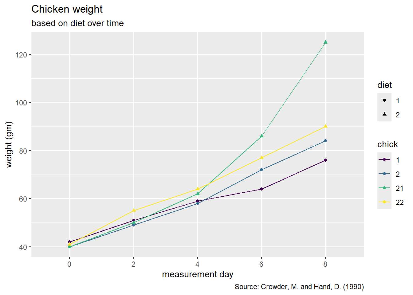

3. Why do we use scale_color_viridis_d() instead of scale_color_viridis_c() in the plot above?

The _d stands for discrete. When we are trying to change the color pallet based on a categorical variable, we need to use _d. If we are trying to change the pallet based on a quantitative variable, we use _c.

4. Why is it important to use scale_color_viridis functions when we create plots?

It’s important for us as statisticians/researchers to make data visualizations that are inclusive as possible for our target audience. The results we create are not worth anything if we can’t articulate it/share it. scale_color_viridis is a function that helps us create a colorblind friendly pallet.

Now is a good time to save, render, and commit/push your changes to GitHub

Note

The “Workflow & formatting” grade is to assess the reproducible workflow. This includes:

• linking all pages appropriately on Gradescope
• putting your name in the YAML at the top of the document
• Pipes %>%, |> and ggplot layers + should be followed by a new line
• Proper spacing before and after pipes and layers
• You should be consistent with stylistic choices, e.g. %>% vs |>
• You must have at least 3 meaningful commits on GitHub

Grading

• Package questions: 15 points
• Flights Hypothesis Test: 30
• Flights simulation: 15 points
• Flights confidence interval: 20 points
• ChickWeights: 25 points
• Workflow + formatting: 10 points
• Total: 115 points