By submitting this exam, I hereby state that I have not communicated with or gained information in any way from my classmates during this exam, and that all work is my own.
Any potential violation of the NC State policy on academic integrity will be reported to the Office of Student Conduct & Community Standards. All work on this exam must be your own.
This exam is due Friday, October 17th, at 11:59PM. Late work is not accepted for the take-home.
You are allowed to ask content clarification questions via email. Any question(s) that give you an advantage to answering a question will not be answered.
This is an individual exam. You may not use your classmates or AI to help you answer the following questions. You may use all other class resources.
Show your work. This includes any and all code used to answer each question. Partial credit can not be earned without any work shown.
Round all answers to 3 digits (ex. 2.34245 = 2.342)
Only use the functions we have learned in class unless the question otherwise specifies. If you have a question about if a function is allowed, please send me an email.
If you are having trouble recreating a plot exactly, you still may earn partial credit if you recreate the plot partially.
You must have at least 3 meaningful commits on your exam1 repo. If you do not, you will lose Workflow and Formatting points.
Do not forget to render after each question! You do not want to have rendering issues close to the due date.
Reminder: Unless you are recreating a plot exactly, all plots should have appropriate labels and not have any redundant information.
Reminder: The phrase “In a single pipeline” means not stopping / having no breaks in your code. An example of a single pipeline is:
Reminder: Use help files! You can access help files for functions by typing ?function.name into your Console.
Good luck!
How to turn your exam
The exam is turned in exactly how you have been turning in homework, via Gradescope. You can find the Gradescope exam1 button on our Moodle page, or go to gradescope.com. Please remember to select your pages correctly when turning in your assignment. For more information, please see on Moodle: Submit Homework on the Gradescope Website.
How to format your Exam
You are asked to format your exam exactly how you would format your homework assignment.
For each question (ex. Question 1), put a level two (two pound signs) section header with the name of the question.
For questions with multiple parts (ex. a, b, c), please put these labels in bold as normal text.
For example…
Question 1
a
Exam Start
Packages
You will need the following packages for the exam.
Hide the all the unnecessary text (not the code itself) using the appropriate code chunk argument for the packages code chunk. You do not need to include any text to answer this question (just hide all the extra text). Hint: You can find a list of these arguments here in the Options available for customizing output include: towards the top.
For question 2, we will be using the following variables:
flight_distance - distance in miles
customer_type - categorized as either Disloyal Customer or Loyal Customer
A disloyal customer is a customer who stops flying from the airline. A loyal customer is someone who continues flying with the airline. You are specifically interested in miles traveled, and if this varies by customer type.
Use the order of subtraction loyal - disloyal. These data are a random sample of all flights from the year 2007.
For this question, you are asked to conduct a hypothesis test to see if there is a difference between the mean distance in miles traveled for different types of customers.
Label your variables as either explanatory/response, and categorical/quantitative, below.
Report your sample mean for each group (using R code) below. Then, write out exactly what your sample statistic is in proper notation.
Write our your null and alternative hypothesis in proper notation.
Can we justify conducting a t test? Show your work below.
Regardless of your answer to part d, we are going to conduct a t-test to test your null and alternative hypotheses in part c. First, calculate your t-statistic below. Show your work.
Use the appropriate R function to calculate your p-value.
Interpret your p-value in the context of the problem. This is different than writing a decision and conclusion. Use the p-value’s definition.
Would you expect a 95% confidence interval to contain the value of 0? Why or why not? Be specific.
Up to this point, we have only been conducting theory based hypothesis testing (z and t-tests). However, we can also use simulation techniques to test our hypotheses. To learn more about this, please read the following Chapters of our textbook:
The key difference between theoretical and simulation based inference is how we determine the null distribution. In theoretical methods, we standardize our sample statistic, and use a t-distribution.
In randomization tests, we empirically construct the null distribution via simulation.
In as much detail as possible, describe the simulation scheme for testing your hypotheses in Question 2. That is, describe how we simulate the null distribution. In your explanation, please include:
– What do we assume to be true
– How is one observation on this simulated null distribution created
Hint: please use the information below in your description.
Now is a good time to save, render, and commit/push your changes to GitHub
Question 4: Flights confidence interval
In this question, you are going to create a theory based 90% confidence interval for the scenario described in Question 2.
Using R, calculate your appropriate t* multiplier.
Now, report your margin of error. Show your work.
Now, report your 90% confidence interval and interpret your 90% confidence interval in the context of the problem.
Discuss one benefit and disadvantage of making an 80% confidence interval instead of a 90% confidence interval.
Now is a good time to save, render, and commit/push your changes to GitHub
Question 5: ChickWeights
For this question, we are going to use a chickweight data set. This is a data set that has data from an experiment of the effect of diet on early growth of baby chickens. Please read in the following data below.
Data
The data key can be seen below:
variable name
description
time
The week in which the measurement was taken (0, 2, 4, 6, 8).
chick
ID number (1, 2, 21, 22)
diet
type of diet(1, 2)
weight
body weight of the chick (gm)
The data can be read in below. Note that we can use as.factor() to make sure R is treating a variable as a category.
Please copy this code an include it in your assignment to read in the data for this question.
# A tibble: 5 × 2
  time   mean
  <fct> <dbl>
1 0      40.8
2 2      51.2
3 4      60.8
4 6      74.8
5 8      93.8
As researchers, it’s critical that you demonstrate your ability to learn and implement new computing skills. In part b, you are going to demonstrate your ability to build upon your existing computing R/statistics skills.
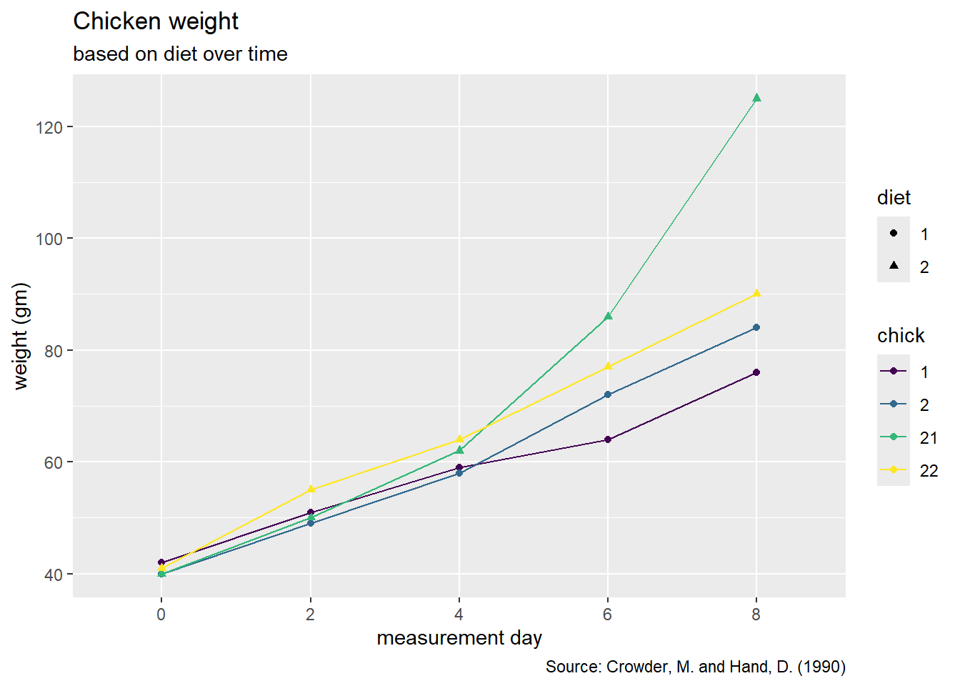
Please recreate the following graph below.
As a reminder, a list of geoms in the tidyverse package can be found here.
Hint: Go to the reference above and look for the geom that connects observations with a line.
Hint: To recreate this plot, we need to specify a group = variable.name to tell R which observations we want to connect to each other in the aes() function.