Warning: package 'tidyverse' was built under R version 4.4.3
Warning: package 'ggplot2' was built under R version 4.4.3
Warning: package 'tibble' was built under R version 4.4.3
Warning: package 'tidyr' was built under R version 4.4.3
Warning: package 'purrr' was built under R version 4.4.3
Warning: package 'dplyr' was built under R version 4.4.3
Warning: package 'stringr' was built under R version 4.4.3
── Attaching core tidyverse packages ──────────────────────── tidyverse 2.0.0 ──
✔ dplyr     1.1.4     ✔ readr     2.1.5
✔ forcats   1.0.0     ✔ stringr   1.5.1
✔ ggplot2   3.5.2     ✔ tibble    3.3.0
✔ lubridate 1.9.3     ✔ tidyr     1.3.1
✔ purrr     1.1.0
── Conflicts ────────────────────────────────────────── tidyverse_conflicts() ──
✖ dplyr::filter() masks stats::filter()
✖ dplyr::lag()    masks stats::lag()
ℹ Use the conflicted package (<http://conflicted.r-lib.org/>) to force all conflicts to become errors
Bumba or Kiki
This is created with fake data that may not exactly match the class recording
How well can humans distinguish one “Martian” letter from another? In today’s activity, we’ll find out. When shown the two Martian letters, kiki and bumba, answer the poll….
Next, write down the number of people that thought option 1 was Bumba. Write down how many people thought option 2 was Bumba.
Option 1: 85
Option 2: 15
The question is: “Which letter is Bumba”
Option 1
Once it’s revealed which optinon is correct, please write our sample statistic below.
\(\hat{p} = \frac{85}{100}\)
Let’s write out the null and alternative hypothesis below. Underneath this, write out what our population parameter is…
Ho: \(\pi = .5\)
Ha: \(\pi > .5\)
Check assumptions
– Independence
– Normality
I’m going to assume that all observations are independent from each other. That is, one observation does not influence the other.
We check normality with success and failures! We need to see at least 10 successes and 10 failures under the assumption of the null hypothesis.
.5 * 100 = 50 > 10
.5 * 100 = 50 > 10
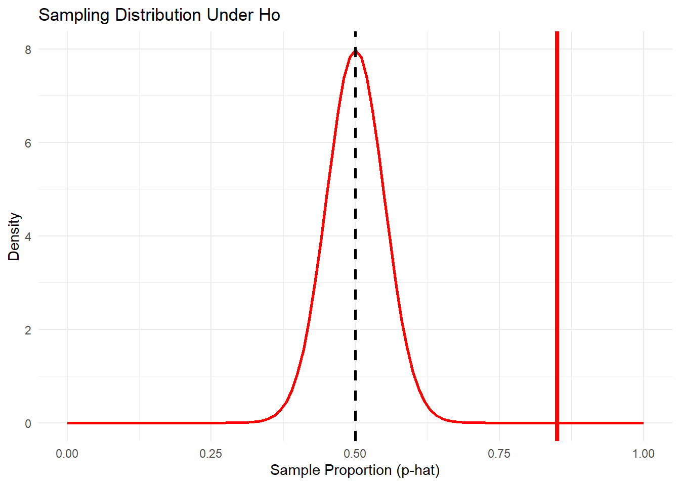
Sampling Distribution
Take a look at the following code. Adjust the sample size according to our class size and run the code.
The following code below is here to help us visualize the sampling distribution of our statistic under the assumption of the null hypothesis.
The goal of this is not to learn the code. The goal of this is to develop a clear foundational understanding about hypothesis testing + p-values.
Please change the sample size and statistic R objects below, and run the code to visualize the p-value.
p_hat<-.85# Sample statisticn<-100# Sample sizep<-0.5# Null value (population proportion)# Calculate the standard error of the sampling distributionstandard_error<-sqrt(p*(1-p)/n)# Create a data frame for the shaded area to the right of p-hatshade_data<-data.frame( x =seq(p_hat, p+4*standard_error, length.out =100))shade_data$y<-dnorm(x =shade_data$x, mean =p, sd =standard_error)# Plot only the theoretical normal curveggplot(data =NULL)+# We can use NULL when there is not an explicit data set# Add the theoretical normal curvestat_function(fun =dnorm, args =list(mean =p, sd =standard_error), color ="red", linewidth =1)+# Shade the area to the right of p-hatgeom_ribbon(data =shade_data, aes(x =x, ymin =0, ymax =y), fill ="red", alpha =0.5)+# Add a vertical line for the mean of the distributiongeom_vline(xintercept =p, color ="black", linetype ="dashed", linewidth =1)+# Add a vertical line for the p-hatgeom_vline(xintercept =p_hat, color ="red", linetype ="solid", linewidth =1.5)+# Add labels and a titlelabs( title ="Sampling Distribution Under Ho", x ="Sample Proportion (p-hat)", y ="Density")+theme_minimal()+# Manually set the x-axis limits to show the full curvexlim(0, 1)
z-distribution
Let’s calculate this p-value using a z-test (as one typically does). Let’s do the calculation below!
Interpret the p-value in the context of the problem.
The probability of observing a sample proportion of .85, or something larger, given the true proportion of students who guess Bumba correctly is .5, is < 0.001.
Decisions and conclusions
Write an appropriate decision and conclusion below. Let’s use \(\alpha\) = 0.05. Before writing a decision and conclusion, let’s talk about \(\alpha\)….
Based on a really small p-value, we reject the null hypothesis, and conclude that the true proportion for students who guess Bumba correctly is actually larger than 50%.