Mean Penguins: Solutions
Packages
Penguins
Includes measurements for penguin species, island in Palmer Archipelago, size (flipper length, body mass, bill dimensions), and sex. The data set is called penguins, and is in the palmerpenguins package. In this activity, we are going to perform a hypothesis test, and calculate a confidence interval for body_mass_g.
Specifically, we are going to look at Gentoo penguins. It is assumed that Gentoo penguins historically weigh, on average, 6500 grams. You want to test if the Gentoo penguins on an island in Palmer Archipelago, are different than what is historically known. For this activity, you may assume that the penguins in this data set are independent from one another. You may assume \(\alpha = 0.05\) for this question.
First, let’s clean up the data set to only include Gentoo penguins. Comment the code below.
# A tibble: 123 × 8
   species island bill_length_mm bill_depth_mm flipper_length_mm body_mass_g
   <fct>   <fct>           <dbl>         <dbl>             <int>       <int>
 1 Gentoo  Biscoe           46.1          13.2               211        4500
 2 Gentoo  Biscoe           50            16.3               230        5700
 3 Gentoo  Biscoe           48.7          14.1               210        4450
 4 Gentoo  Biscoe           50            15.2               218        5700
 5 Gentoo  Biscoe           47.6          14.5               215        5400
 6 Gentoo  Biscoe           46.5          13.5               210        4550
 7 Gentoo  Biscoe           45.4          14.6               211        4800
 8 Gentoo  Biscoe           46.7          15.3               219        5200
 9 Gentoo  Biscoe           43.3          13.4               209        4400
10 Gentoo  Biscoe           46.8          15.4               215        5150
# ℹ 113 more rows
# ℹ 2 more variables: sex <fct>, year <int>
Exploratory data analysis
Before we conduct our hypothesis test, let’s explore the data. Below, calculate the mean value of body_mass_g, and make an appropriate visualization to explore the shape of the data.
gen_data |>
  ggplot(
    aes(x = body_mass_g)
  ) +
  geom_histogram()
`stat_bin()` using `bins = 30`. Pick better value with `binwidth`.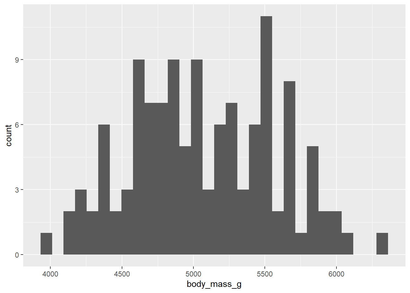
# A tibble: 1 × 1
  count
  <int>
1   123
Hypothesis Testing
Write out your null and alternative hypothesis below in both words and proper notation:
The true mean body mass (g) of Gentoo penguins is equal to 6500
\(Ho: \mu = 6500\)
The true mean body mass (g) of Gentoo penguins is different from 6500
\(Ho: \mu \neq 6500\)
List out, and check your assumptions below.
– Independence
– Normality
The shape of this distribution looks roughly normal! With a large sample size (n > 60), and assuming that these penguins are independent, I feel justifiable to do a theoretical hypothesis test!
Using a t-statistic, calculate your p-value below.
# A tibble: 1 × 3
   mean    sd  size
  <dbl> <dbl> <int>
1 5076.  504.   123
\(t = \frac{5076 - 6500}{504/\sqrt{123}} = −31.335\)
Why t and not z?
Because we are estimating \(\mu\) with \(\bar{x}\) and also the population standard deviation \(\sigma\) with \(s\)
How does a t distribution differ from a z distribution?
They have the same center, but the t-distribution has more uncertainty on the tails!
Write out an appropriate decision and conclusion in the context of the problem.
pt(-31.335, df = 123, lower.tail = TRUE)*2[1] 1.764128e-60Based on our really small p-value, we would reject the null hypothesis, and have strong evidence to conclude that the true mean body mass (g) for Gentoo penguins is different than 6500.
Confidence intervals
Now, we want to estimate the true mean body mass (g) of Gentoo penguins. Let’s do so below.
As a reminder, our best guess of \(\mu\) is \(\bar{x}\). Let’s quantify the uncertainty around this guess by estimating the standard error around our statistic.
We did this above! The standard error is the same for hypothesis testing and confidence intervals for a quantitative response.
\(\frac{s}{\sqrt{n}}\)
\(\frac{504}{\sqrt{123}} = 45.444\)
Now, calculate the appropriate t*, and calculate a 95% confidence interval. Interpret it below.
qt(.975, df = 122, lower.tail = T)[1] 1.9796\(\bar{x_1}\pm t^* * SE(\bar{x_1})\)
6500 \(\pm\) 1.9796 * 45.444
(6410.039, 6589.961)
We are 95% confident that the true mean body mass of Gentoo penguins (g) is between 6410.039 and 6589.961 grams.
We
Connecting hypothesis testing and confidence intervals
For a two-sided hypothesis test at \(\alpha = 0.05\), we rejected the null hypothesis, AND saw that 0 was not in our confidence interval. This is not by accident. Let’s connect the dots.
Hypothesis Test (Rejection): You reject the null hypothesis \(Ho: \mu = 6500\) if the sample mean is far enough away from the center so that the p-value is < 0.05.
That is, this distance is quantified by the test statistic (t) falling outside the critical region of -1.9794387
A 95% confidence interval is defined as: \(\bar{x} \pm t^* * SE\)
This interval captures all the values of \(\mu\) that would not lead to the rejection of the null hypothesis at \(\alpha = 0.05\)
If the hypothesis test leads you to reject the null hypothesis, it means that the distance between \(\bar{x} and \mu_o\) is greater than the margin of error defined by the 95% CI.