Anova

Post-Hoc analysis Solutions

Packages

library(tidyverse)
library(palmerpenguins)
library(broom)

Creating variables and working with missing values

It’s important to be able to check for, and remove missing values from a data set. You will not be tested on this, but let’s practice this together! Comment through the code below:

penguins |>
  mutate(missing = is.na(bill_length_mm)) |> #make a new variable called missing
  filter(missing == TRUE) # only select rows that have TRUE in the missing variable

# A tibble: 2 × 9
  species island    bill_length_mm bill_depth_mm flipper_length_mm body_mass_g
  <fct>   <fct>              <dbl>         <dbl>             <int>       <int>
1 Adelie  Torgersen             NA            NA                NA          NA
2 Gentoo  Biscoe                NA            NA                NA          NA
# ℹ 3 more variables: sex <fct>, year <int>, missing <lgl>

Saving a new data set

Comment through the code below

peng_filter <- penguins |> # make a new R object called peng_filter
  mutate(missing = is.na(bill_length_mm)) |> # make a missing variable
  filter(missing == FALSE) # only select rows that have FALSE in the missing variable

Note: There are functions like drop_na(): which removes rows containing any NA values. These can be dangerous…

Anova

Now, let’s conduct an ANOVA test between species and bill length. First, let’s check our assumptions.

Normality

The sample = argument within the aes() (aesthetic) function in ggplot2 orders our data on the y-axis. stat_qq_line() maps the theoretical quantiles to our plot.

penguins |>
      ggplot(
        aes(sample = bill_length_mm)) +
      stat_qq() +
      stat_qq_line() +
      facet_wrap(~ species) + # Replace 'Species' with your grouping variable
      labs(title = "QQ Plots of Bill Length by Species",
           x = "Theoretical Quantiles (what we would expect to see from a Z)",
           y = "Ordered data") +
      theme_minimal()

Warning: Removed 2 rows containing non-finite outside the scale range
(`stat_qq()`).

Warning: Removed 2 rows containing non-finite outside the scale range
(`stat_qq_line()`).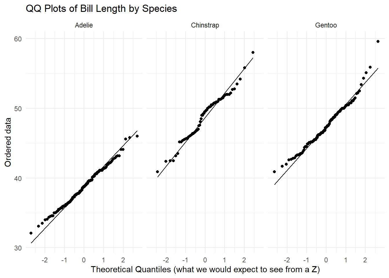

For each of the three species, we see a linear relationship between our ordered data and what we would expect to see from a normal distribution. There is not enough evidence to suggest that the normality assumption is violated.

Equal Variance

Use the appropriate R code below to justify the equal variance assumption. Note: The general rule is the largest standard deviation should not be two times the smallest.

peng_filter |>
  group_by(species) |>
  summarise(mean = mean(bill_length_mm),
            sd = sd(bill_length_mm))

# A tibble: 3 × 3
  species    mean    sd
  <fct>     <dbl> <dbl>
1 Adelie     38.8  2.66
2 Chinstrap  48.8  3.34
3 Gentoo     47.5  3.08

3.34/2.66 < 2

[1] TRUE

Anova

Fill in the blanks below to conduct your test for anova.

anova_model <- aov(bill_length_mm ~ species, data = peng_filter)

summary(anova_model)

             Df Sum Sq Mean Sq F value Pr(>F)    
species       2   7194    3597   410.6 <2e-16 ***
Residuals   339   2970       9                   
---
Signif. codes:  0 '***' 0.001 '**' 0.01 '*' 0.05 '.' 0.1 ' ' 1

We can start working with values when the table is a tibble. We can use the tidy() function from the broom package.

tidy(anova_model)

# A tibble: 2 × 6
  term         df sumsq  meansq statistic   p.value
  <chr>     <dbl> <dbl>   <dbl>     <dbl>     <dbl>
1 species       2 7194. 3597.        411.  2.69e-91
2 Residuals   339 2970.    8.76       NA  NA       

tb <- tidy(anova_model) # save the tibble as tb

tb_species <- tb |>
  filter(term == "species")

tb_species$statistic

[1] 410.6003

tb_species$p.value

[1] 2.694614e-91

You can write in-line code by putting backticks (instead of ” “) around the”r your code here”. Put the R code you want to execute in-line below within your sentence!

Our statistic is 410.600255

Our p-value is rtb_species$p.value`

Tukeys

To conduct Tukeys HSD, run the code below.

TukeyHSD(anova_model)

  Tukey multiple comparisons of means
    95% family-wise confidence level

Fit: aov(formula = bill_length_mm ~ species, data = peng_filter)

$species
                      diff       lwr        upr     p adj
Chinstrap-Adelie 10.042433  9.024859 11.0600064 0.0000000
Gentoo-Adelie     8.713487  7.867194  9.5597807 0.0000000
Gentoo-Chinstrap -1.328945 -2.381868 -0.2760231 0.0088993