        corr
1 -0.4579879Inference for Regression
Dr. Elijah Meyer
NC State University
ST 511 - Fall 2025
2025-11-05
Checklist
– Quiz released this afternoon (due Sunday)
– Homework released Friday (due Friday)
– Statistics experience released
– Expect take-home grades by tonight
– Final Exam is Dec 8th at 3:30 (expect an email this afternoon)
AI
Thinking about your future
– Calculators don’t make you good at math… LLMs don’t make good researchers
– If you work with private data, you can’t use LLMs
– If you only know how to use LLMs, your skillset is not marketable… it’s sloppy (especially in statistics)
– LLMs are trained on a lot of data (some correct/some not). Think of your last Google Search.
AI
Thinking about you as a student
We (very often) don’t use AI as a learning tool, and instead use it as a producer
Once you have the foundation, this tool can really help you
This is an introduction to statistics course (we are building the foundation)
AI
Thinking about you as a student
… and I know how stressed you are with time (I was a student just a couple years ago)
– but this hurts you now
– and hinders where you are going
Warm Up

How can we summarize these data?
Summary statistics
– correlation (r)
– slope + intercept (fit a line)
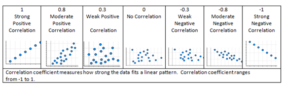
Correlation
In R
Let’s find the correlation coefficient between our two variables
syntax: cor(x, y)
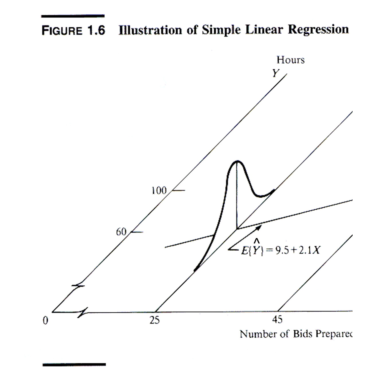
Fit a line
… and talk about the slope and the intercept

The line
Let me (re) introduce you to:
Population level: \(y = \beta_o + \beta_1*x + \epsilon\)
Sample: \(\hat{y} = \hat{\beta_o} + \hat{\beta_1}*x\)
In R
# A tibble: 2 × 5
  term        estimate std.error statistic  p.value
  <chr>          <dbl>     <dbl>     <dbl>    <dbl>
1 (Intercept)   23.2      2.11       11.0  4.90e-21
2 Temp          -0.170    0.0269     -6.33 2.64e- 9
– Prediction
– Interpretation
Why mean response?
Statistical Inference
We can also test for a linear relationship between x and y…
What would the null and alternative hypotheses be?
Null and alternative
\(H_o: \beta_1\) = 0
\(H_a: \beta_1 \neq 0\)
Assumptions
– Independence (we know how to check this)
– Linear relationship (two ways to check this)
– Equal Variance (new way to check this)
– Normality or residuals (we know how to check this)
Independence
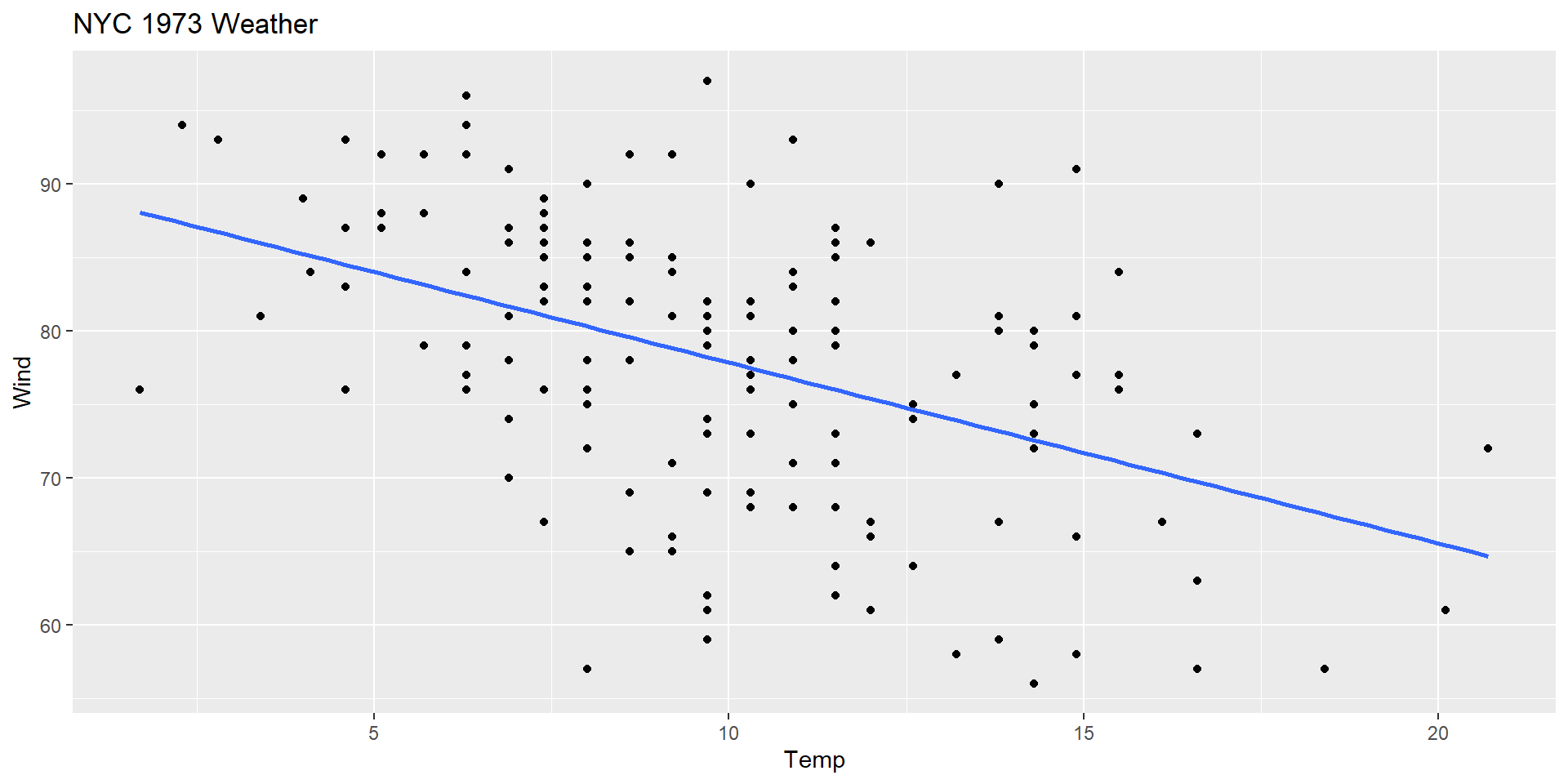
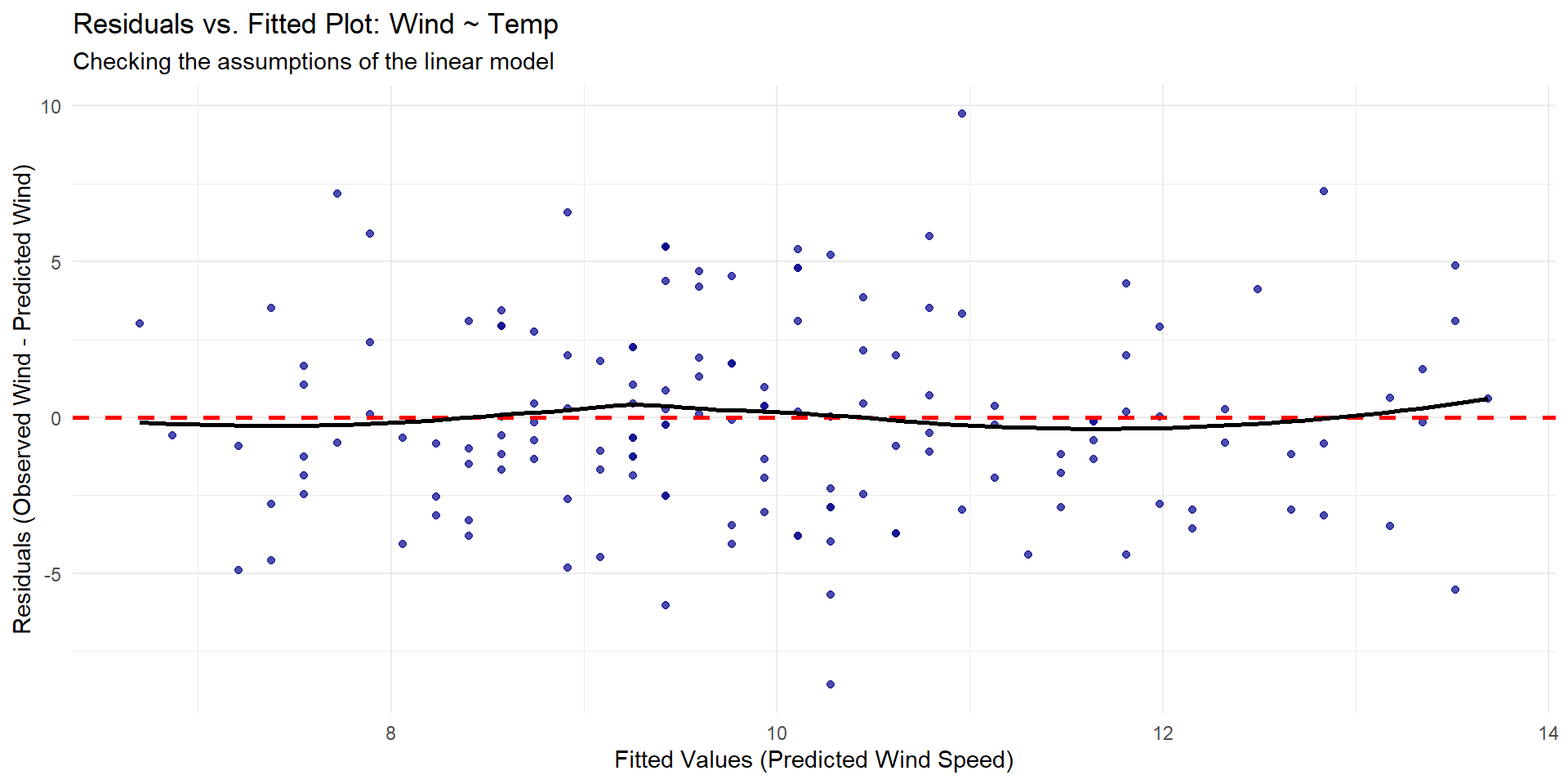
Linear relationship
Does it make sense?
Residual vs Fitted (Predicted)

Violation of linearity
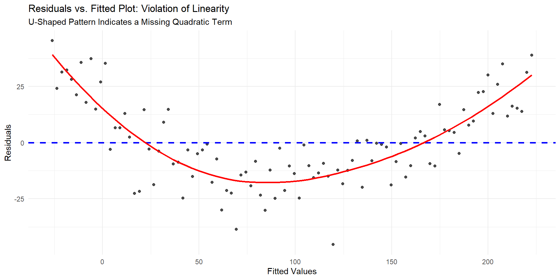
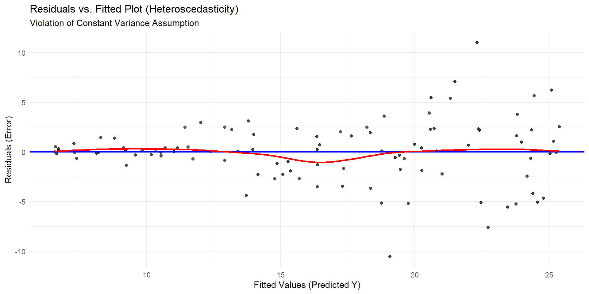
Residual vs Fitted (Predicted)
Checking Equal Variance!
Violation of Equal Variance
In Summary

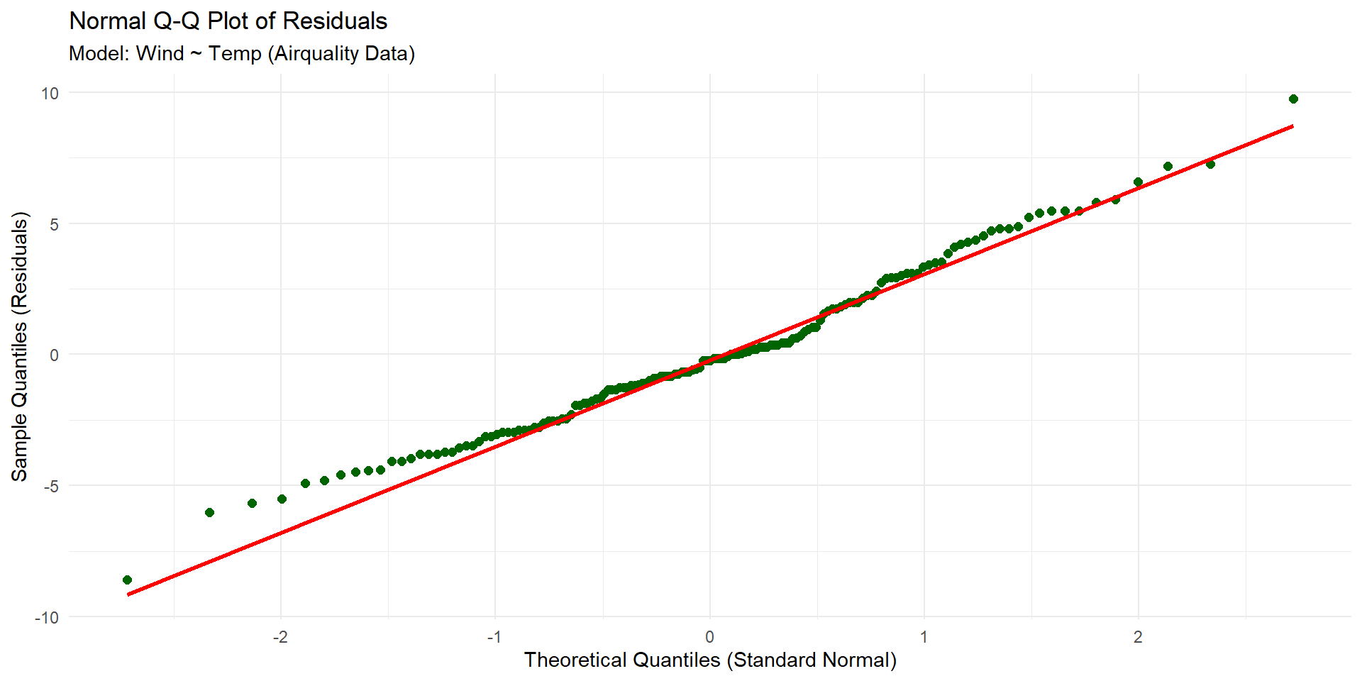
Normality
We think about our sample size and also look at Normal Q-Q plots!
In R
Test statistic
t
… (yes this is the entire slide….)
Test statistic
\[t = \frac{\hat{\beta}_1 - \beta_{\text{null}}}{\text{SE}(\hat{\beta}_1)}\]
Standard Error
\[\text{SE}(\hat{\beta}_1) = \sqrt{\frac{\text{Unexplained Variation in } Y \text{ (due to error)}}{\text{Variation/Spread in } X \text{}}}\]
\[\text{SE}(\hat{\beta}_1) = \sqrt{\frac{\hat{\sigma}^2}{\sum_{i=1}^{n} (X_i - \bar{X})^2}}\]
\[\hat{\sigma}^2 = \frac{\text{RSS}}{n - 2}\]
\[\hat{\sigma}^2 = \frac{\sum_{i=1}^{n} (Y_i - \hat{Y}_i)^2}{n-2}\]
Output
| term | estimate | std.error | statistic | p.value |
|---|---|---|---|---|
| (Intercept) | 23.234 | 2.112 | 10.999 | 0 |
| Temp | -0.170 | 0.027 | -6.331 | 0 |
And this t-statistic follows a t-distribution with n-2 degrees of freedom (-2 because we estimate the population slope and intercept)
– Recreate the statistic
– Draw out what the p-value would look like
What does all of this mean?
Confidence intervals
We can calculate two types of confidence intervals:
– Confidence interval for the mean response (what we will cover)
– Confidence interval for the slope (next time)
– Prediction interval for a brand new observation
Output
| term | estimate | std.error | statistic | p.value |
|---|---|---|---|---|
| (Intercept) | 23.234 | 2.112 | 10.999 | 0 |
| Temp | -0.170 | 0.027 | -6.331 | 0 |
Suppose I want to predict the true mean Wind (mph) for when the Temp is 17 degrees.
Do it!
Do you think this is the true value?
Response
\(\hat{\mu_y} \pm t^* * SE_\hat{\mu_y}\)
Standard Errors
\(X_\text{given}\) = What we set x equal to
\[\text{SE}_{\hat{\mu}_{Y}|X_g} = \sqrt{\hat{\sigma}^2 \left[\frac{1}{n} + \frac{(X_\text{given} - \bar{X})^2}{\sum_{i=1}^{n} (X_i - \bar{X})^2}\right]}\]
Terms
The term \(\frac{1}{n}\) accounts for the general uncertainty in estimating the intercept
The term \(\hat{\sigma}^2\) in the outer square root represents the uncertainty around our prediction.
\(\left(\frac{(X_{\text{given}} - \bar{X})^2}{\sum_{i=1}^{n} (X_i - \bar{X})^2}\right)\) accounts for the uncertainty introduced by the slope (\(\hat{\beta}_1\)).
Review
What happens to these intervals when…
– n goes up?
– Confidence level goes down?