Multiple Linear Regression: Inference

Dr. Elijah Meyer

NC State University
ST 511 - Fall 2025

2025-11-12

Checklist

– Quiz released Wednesday (due Sunday)

– Homework has been assigned (due Sunday)

– Statistics experience released

– Final Exam is Dec 8th at 3:30

For those who have indicated a university excused reason to miss, you should have received an email

Warm-up

What’s the difference between:

– Simple linear regression

– Multiple linear regression (additive)

– Multiple linear regression (interaction)

Simple linear regression (SLR)

– Quantitative response (Y)

– Single quantitative explanatory (X)

… note: you can use linear models with a categorical explanatory variable, but the math comes out to just doing a t-test / ANOVA

Multiple linear regression (additive)

– Quantitative response (Y)

– > 1 explanatory variable

What’s the assumption of the additive model?

Assumption

The relationship between x and y does not depend on z

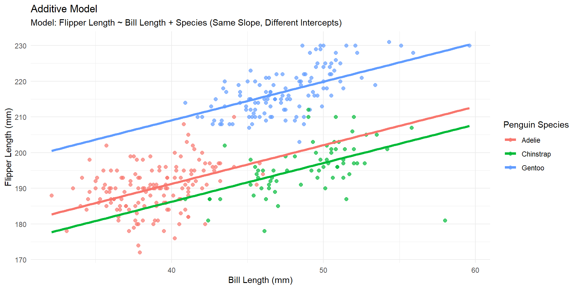
Additive model

Model Output

term	estimate	std.error	statistic
(Intercept)	147.951	4.174	35.447
bill_length_mm	1.083	0.107	10.129
speciesChinstrap	-5.004	1.370	-3.653
speciesGentoo	17.799	1.170	15.216

How do we interpret 1.083?

How do we interpret 17.799?

Interpretations

Holding species constant, for a 1 mm increase in bill length, we estimate an average increase in flipper length of 1.083mm.

Holding bill length constant, we estimate the mean flipper length of Gentoo penguins to be 17.799mm larger than the Adelie penguins.

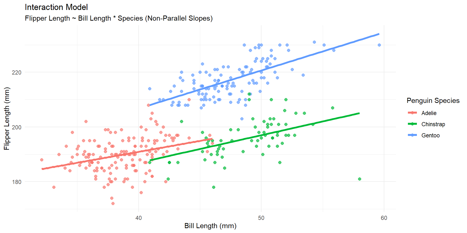
Multiple linear regression (interaction)

Assumption:

The relationship between x and y depends on the values of z

Interaction model

Output

# A tibble: 6 × 5
  term                            estimate std.error statistic  p.value
  <chr>                              <dbl>     <dbl>     <dbl>    <dbl>
1 (Intercept)                      159.        6.90     23.0   4.72e-71
2 bill_length_mm                     0.800     0.178     4.50  9.17e- 6
3 speciesChinstrap                 -12.3      12.5      -0.986 3.25e- 1
4 speciesGentoo                     -7.83     10.6      -0.736 4.63e- 1
5 bill_length_mm:speciesChinstrap    0.207     0.276     0.750 4.54e- 1
6 bill_length_mm:speciesGentoo       0.591     0.246     2.40  1.67e- 2

How do we interpret 0.207?

Interpretation

For a 1 mm increase in bill length, we estimate an average increase in flipper length of 0.207mm more for Chinstrap than Adelie penguins, holding all OTHER variables constant

Ex. Holding Gentoo constant at 0.

Questions ?

Assumptions

– When fitting linear regression models… we also need to think about multicolinearity

Multicolinearity example

We will work with fake data to demonstrate this concept.

# A tibble: 100 × 3
        y  var1  var2
    <dbl> <dbl> <dbl>
 1 -7.72  12.7  12.1 
 2 -2.44   8.87  8.51
 3  0.168 10.7   9.15
 4 -3.60  11.3  11.1 
 5 -2.94  10.8   9.39
 6 -3.16   9.79  8.86
 7 -4.19  13.0  11.5 
 8 -2.74   9.81  8.77
 9 -5.75  14.0  12.7 
10 -2.28   9.87  8.95
# ℹ 90 more rows

Multicolinearity example

# A tibble: 2 × 5
  term        estimate std.error statistic  p.value
  <chr>          <dbl>     <dbl>     <dbl>    <dbl>
1 (Intercept)    6.04     0.810       7.45 3.65e-11
2 var1          -0.791    0.0788    -10.0  1.01e-16

Multicolinearity example

# A tibble: 2 × 5
  term        estimate std.error statistic  p.value
  <chr>          <dbl>     <dbl>     <dbl>    <dbl>
1 (Intercept)    6.89     0.634       10.9 1.51e-18
2 var2          -0.978    0.0687     -14.2 1.38e-25

Multicolinearity example

# A tibble: 3 × 5
  term        estimate std.error statistic  p.value
  <chr>          <dbl>     <dbl>     <dbl>    <dbl>
1 (Intercept)     5.72     0.503     11.4  1.56e-19
2 var1            1.77     0.210      8.44 3.06e-13
3 var2           -2.83     0.225    -12.5  4.91e-22

Adding two variables that are near identical (highly correlated) provides instability in the estimates, p-values, etc.

How to check

– You can calulate correlation coefficients between all your predictors

– You can calculate things variance inflation factors (not covered, but I’ll post something for you!)

Questions ?

Research Question

Is there evidence of an interaction?

Is a variable worth including in our model?

Last time

Simple linear regression

\(H_o: \beta_1 = 0\)

\(H_o: \beta_1 \neq 0\)

Now

We can test between simple and multiple linear regression (let’s start with this)

We can test between different types of multiple linear regression models

Hypothesis Test

\[fl = \beta_o + \beta_1*bill + \epsilon \]

\[fl = \beta_o + \beta_1*bill + \beta_2*Chin + \beta_3*Gentoo + \epsilon \]

What would be my null and alternative hypothesis to test and see if the multiple linear regression model is worth it?

Regression

\(H_o\): \(\beta_2 = \beta_3 = 0\)

\(H_a\): At least one of the betas differ from zero

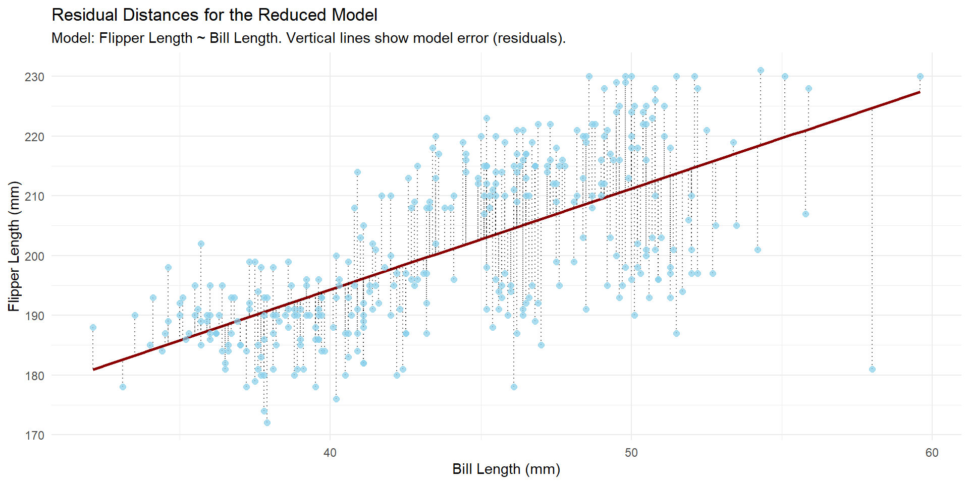
The idea is to…

…see if the reduction in unexplained variance (the reduction in Residual Sum of Squares, RSS) when moving from \(Model_\text{reduced}\) to \(Model_\text{Full}\) is statistically significant.

or, is species a good predictor/worth it to include!

This sounds like something we’ve done before……

ANOVA

\(\mathbf{F} = \frac{\frac{\text{SS}_{\text{Between}}}{k - 1}}{\frac{\text{SS}_{\text{Within}}}{N - k}}\)

Now let’s do this with regression…

Test Statistic

\(F = \frac{(\text{RSS}_R - \text{RSS}_F) / (\text{df}_R - \text{df}_F)}{\text{MSE}_F}\)

\(\text{df}_F = n - k_F - 1\); n is our sample size; k is the number of predictors

\(\text{df}_R = n - k_R - 1\); n is our sample size; k is the number of predictors

Visually

Assumptions

Check for both models!

– Independence

– Linearity

– Normality of residuals

– Equal Variance

… and they need to be nested models

Independence

How do we check it?

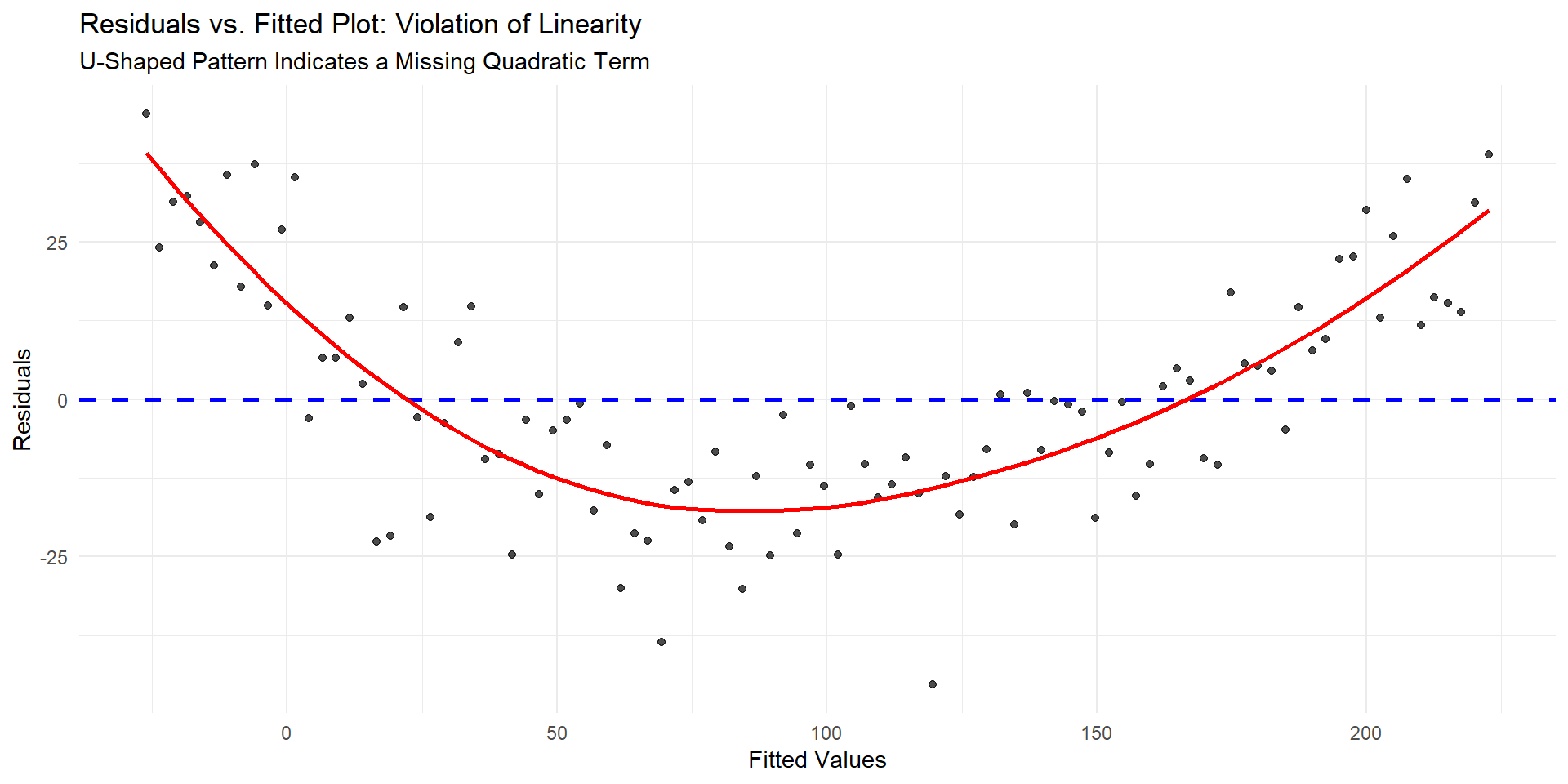
Linearity and Equal Variance

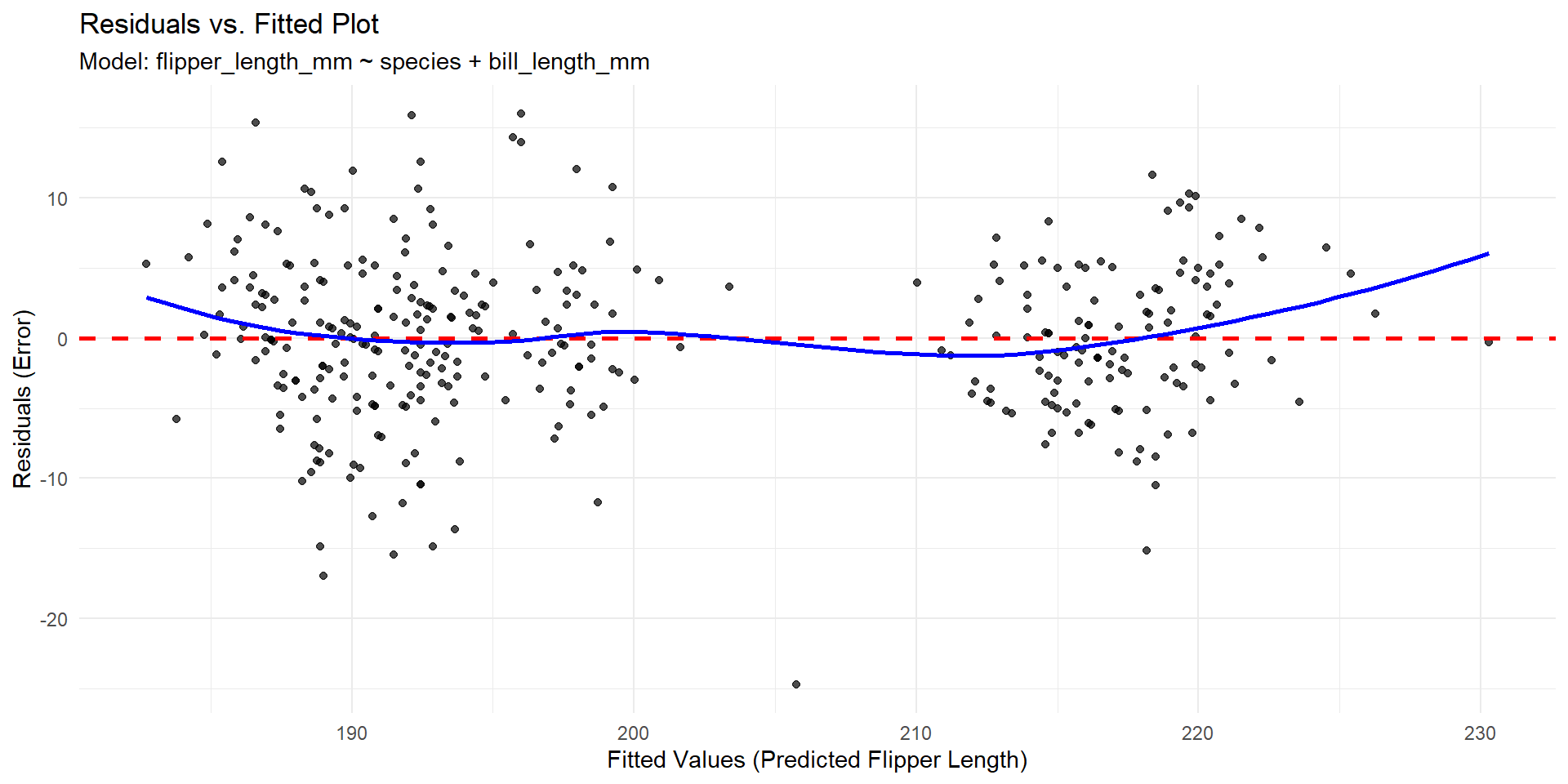
Violation of Equal Variance

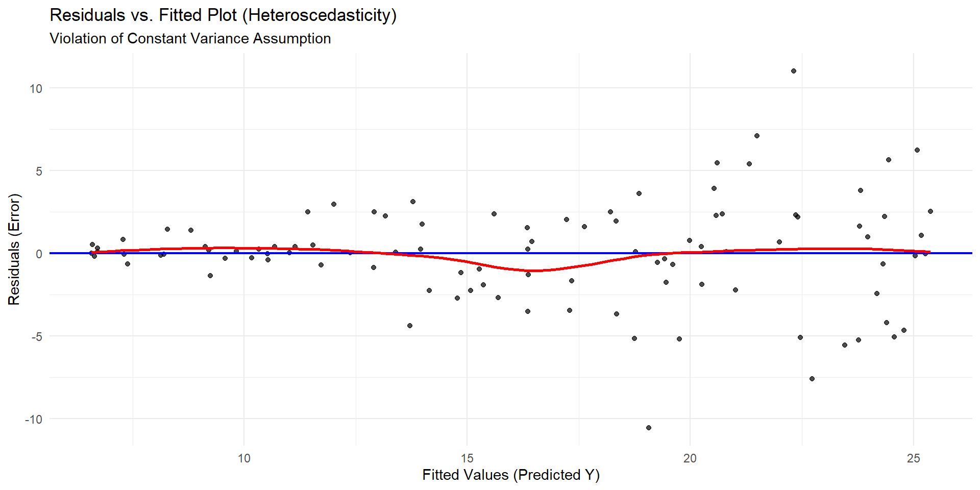
Violation of linearity

Normality

we have a large sample size!

Nested models

What does it mean to be nested?

We can perform transformations to help fix equal variance / normality (not covered, but I can post something about it)

You need to check assumptions for both models

Output

Analysis of Variance Table

Model 1: flipper_length_mm ~ bill_length_mm
Model 2: flipper_length_mm ~ bill_length_mm + species
  Res.Df   RSS Df Sum of Sq      F    Pr(>F)    
1    340 38394                                  
2    338 11471  2     26923 396.64 < 2.2e-16 ***
---
Signif. codes:  0 '***' 0.001 '**' 0.01 '*' 0.05 '.' 0.1 ' ' 1

The DF column difference in residual degrees of freedom between the two adjacent models being compared. This is the numerator degrees of freedom for the \(F\)-test. The denomenator degrees of freedom is the Residual degrees of freedom from the full model (338).

The 26923 is the reduction in the Residual Sum of Squares (RSS) from the reduced to full model.

Our p-value comes from a F-distribution with 2 and 338 degrees of freedom.

In R

model_reduced <- lm(flipper_length_mm ~ bill_length_mm, data = penguins)

model_full <- lm(flipper_length_mm ~ bill_length_mm + species, data = penguins)

anova(model_reduced, model_full)

Analysis of Variance Table

Model 1: flipper_length_mm ~ bill_length_mm
Model 2: flipper_length_mm ~ bill_length_mm + species
  Res.Df   RSS Df Sum of Sq      F    Pr(>F)    
1    340 38394                                  
2    338 11471  2     26923 396.64 < 2.2e-16 ***
---
Signif. codes:  0 '***' 0.001 '**' 0.01 '*' 0.05 '.' 0.1 ' ' 1

What can we conclude?

Additive vs Interaction model

\[fl = \beta_o + \beta_1*bill + \beta_2*Chin + \beta_3*Gentoo + \epsilon \]

\[fl = \beta_o + \beta_1*bill + \beta_2*Chin + \beta_3*Gentoo + \beta_4*bill*Chin +\]

\[\beta_5*bill*Gentoo + \epsilon \]

Visually (interaction)

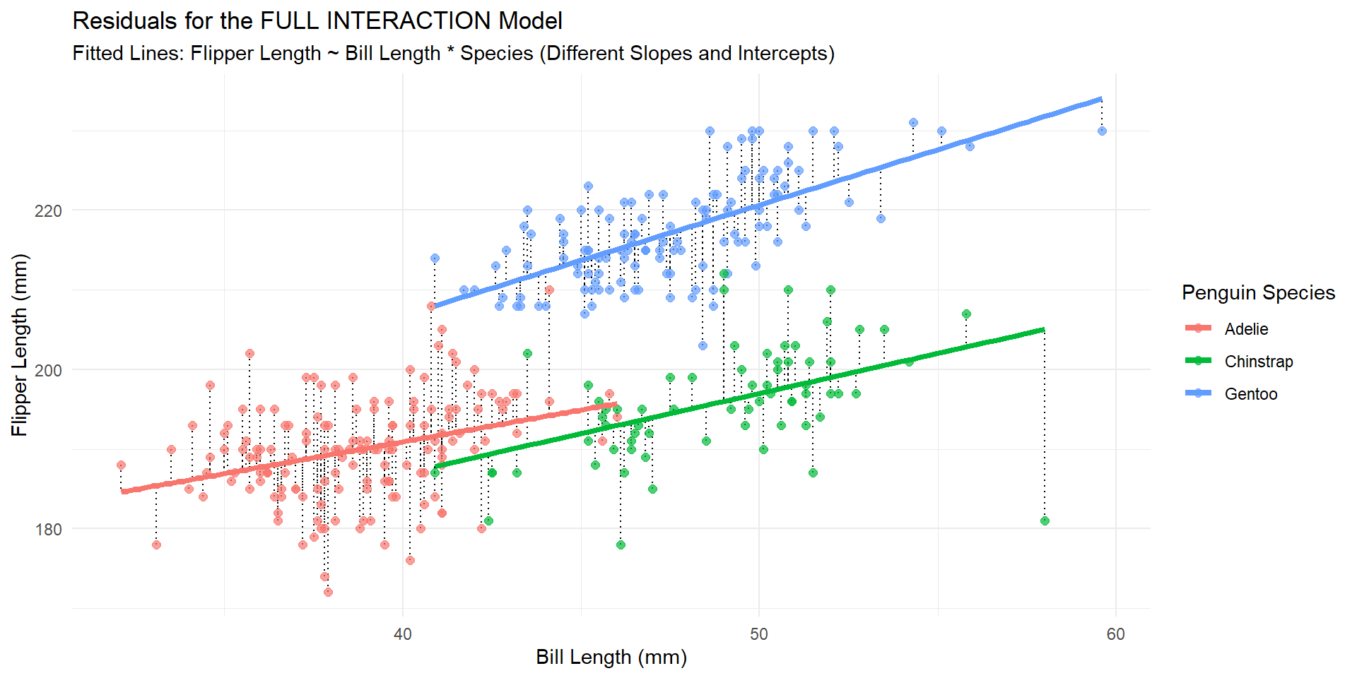
Visually (additive)

Test Statistic

\[F = \frac{(\text{RSS}_R - \text{RSS}_F) / (\text{df}_R - \text{df}_F)}{\text{MSE}_F}\]

Test statistic

Analysis of Variance Table

Model 1: flipper_length_mm ~ bill_length_mm + species
Model 2: flipper_length_mm ~ bill_length_mm * species
  Res.Df   RSS Df Sum of Sq      F  Pr(>F)  
1    338 11471                              
2    336 11272  2    199.66 2.9759 0.05235 .
---
Signif. codes:  0 '***' 0.001 '**' 0.01 '*' 0.05 '.' 0.1 ' ' 1