Finish Difference in Proportions
and intro to Single Mean
NC State University
ST 511 - Fall 2025
2025-09-29
Checklist
– HW-3 due October 5th
– Are you keeping up with the prepare material?
– single_mean repo today. Please clone this now!
We will finish difference in proportions, and then start this today.
Exam-1
It’s coming up
– in-class (October 8th)
– take-home (Due October 17th)
Questions?
Last Time
A pharmaceutical company is conducting a clinical trial to test the effectiveness of a new drug for a common illness. They randomly assign participants to one of two groups
Group 1 (New Drug): Out of 200 patients, 160 recovered from the illness.
Group 2 (Placebo): Out of 180 patients, 126 recovered from the illness.
\(H_o: \pi_n - \pi_p = 0\)
\(H_o: \pi_n - \pi_p > 0\)
\(\hat{p_n} - \hat{p_p} = .1\)
z and p-value
\(Z = \frac{.1 - 0}{\sqrt{.774*.226(\frac{1}{200} + \frac{1}{180})}}\) = 2.327
Decission and Conclusion
Because or p-value is < \(\alpha\), we reject the null hypothesis, and have strong evidence to conclude that the true proportion of patients who recovered from the illness taking the new drug is larger than those who took the placebo.
Let’s estimate it!
Confidence intervals and hypothesis testing
Typically, you report both in research.
Let’s estimate what \(\pi_n - \pi_p\) actually is!
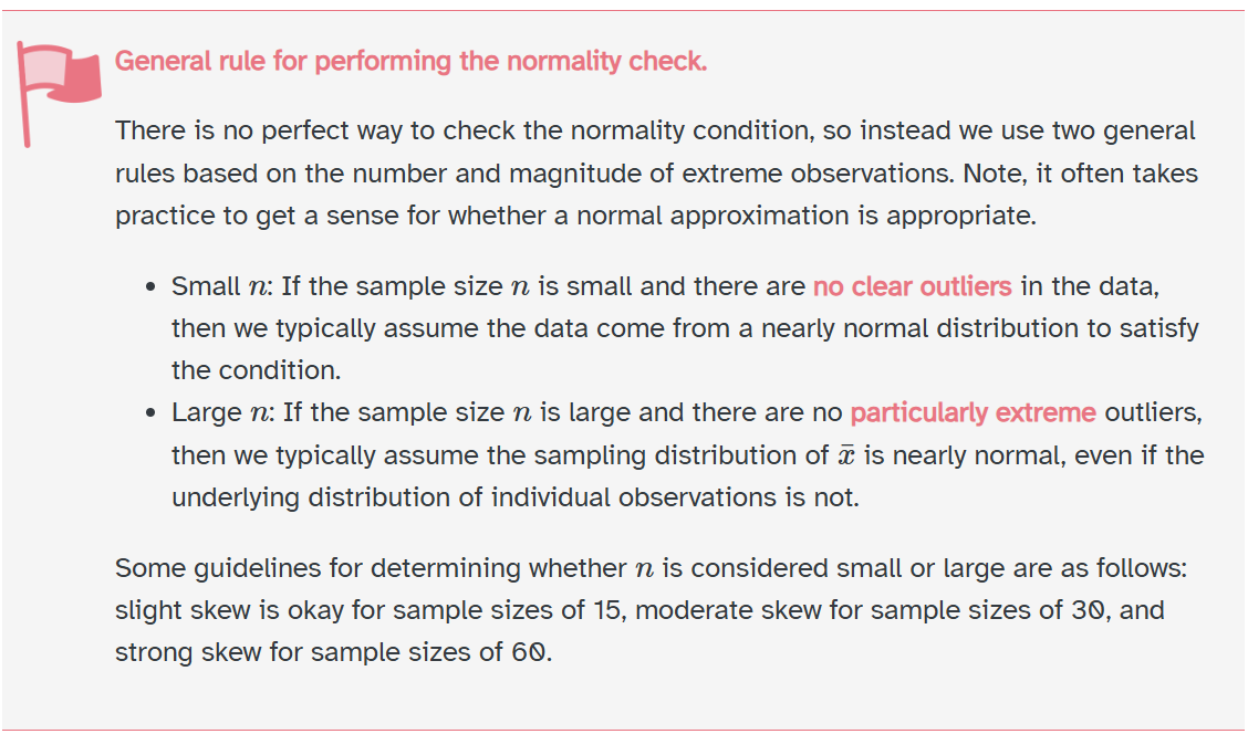
Assumptions
Independence (check)
Success-failure (how is this different than hypothesis testing?)
Success-failure
\(\hat{p_n} * n1 > 10\)
\((1 - \hat{p_n}) * n1 > 10\)
\(\hat{p_p} * n2 > 10\)
\((1 - \hat{p_p}) * n2 > 10\)
Success-failure
\(.8 * 200 > 10\)
\(.2 * 200 > 10\)
\(.7 * 180 > 10\)
\(.3 * 180 > 10\)
Confidence Interval
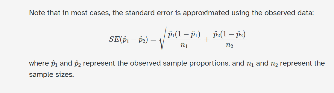
Confidence Interval
\(\sqrt{\frac{.8 *.2}{200} + \frac{.7*.3}{180}}\) = 0.00443
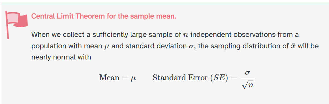
Now, let’s use our best guess for \(\pi_n - \pi_p\) with our estimated standard error to approximate the sampling distribution!
Plot
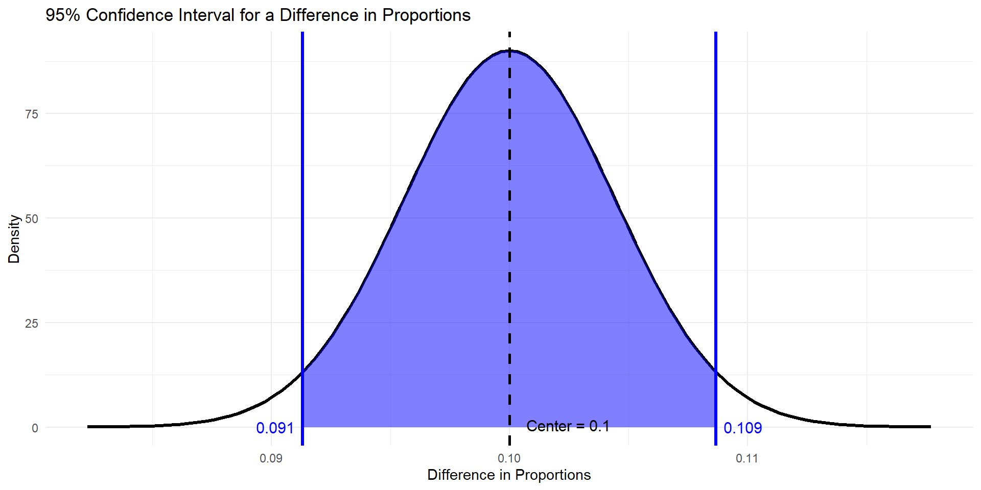
\(.1 + .00443 * 1.96\)
\(.1 - .00443 * 1.96\)
Interpret
We are 95% confident that the true proportion of patients who took the new drug and recovered is 0.091 to 0.109 HIGHER than the true proportion of patients who took the placebo and recovered.
New things:
– Direction!
Questions
single mean ae
t vs normal
– there are infinite t-distributions vs one-normal distribution
– t-distribution approaches a normal distribution when df goes up!
What are degress of freedom?
Degrees of freedom for a t-distribution refer to the number of independent pieces of information that are available to estimate a parameter.
In the context of the t-distribution, the degrees of freedom are a parameter that determines the shape of the distribution
What are degress of freedom?
If our sample size is 124, our degrees of freedom would be 123.
For example, if you have n = 124, once you know the values of 123 observations, the 124th observation must be whatever makes the math equal \(\bar{x} = 124\)
We have 123 independent pieces of information, and one dependent piece of information.
why t
In essence, the degrees of freedom correct for the uncertainty introduced when estimating the population standard deviation using the sample standard deviation when working with a quantitative variable.
The standard error of the sampling distribution is known for hypothesis tests with categorical data, derived from \(\pi_o\), so we don’t correct with t, and use the standard normal distribution.
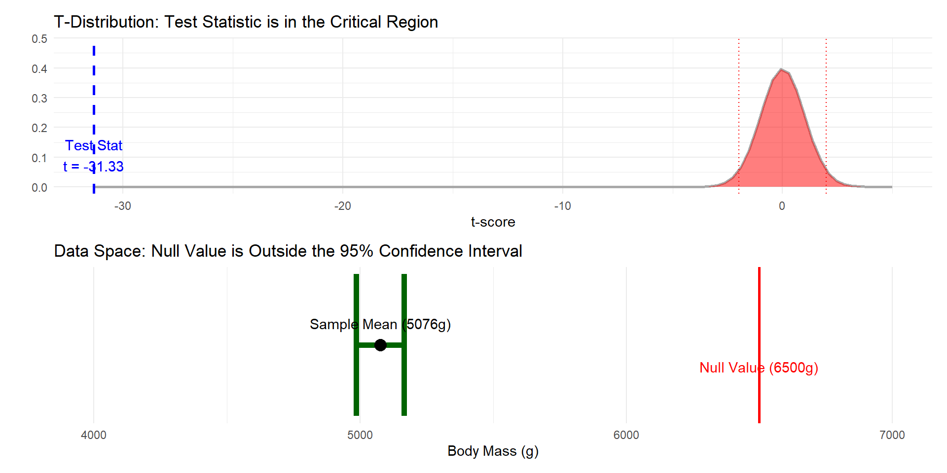
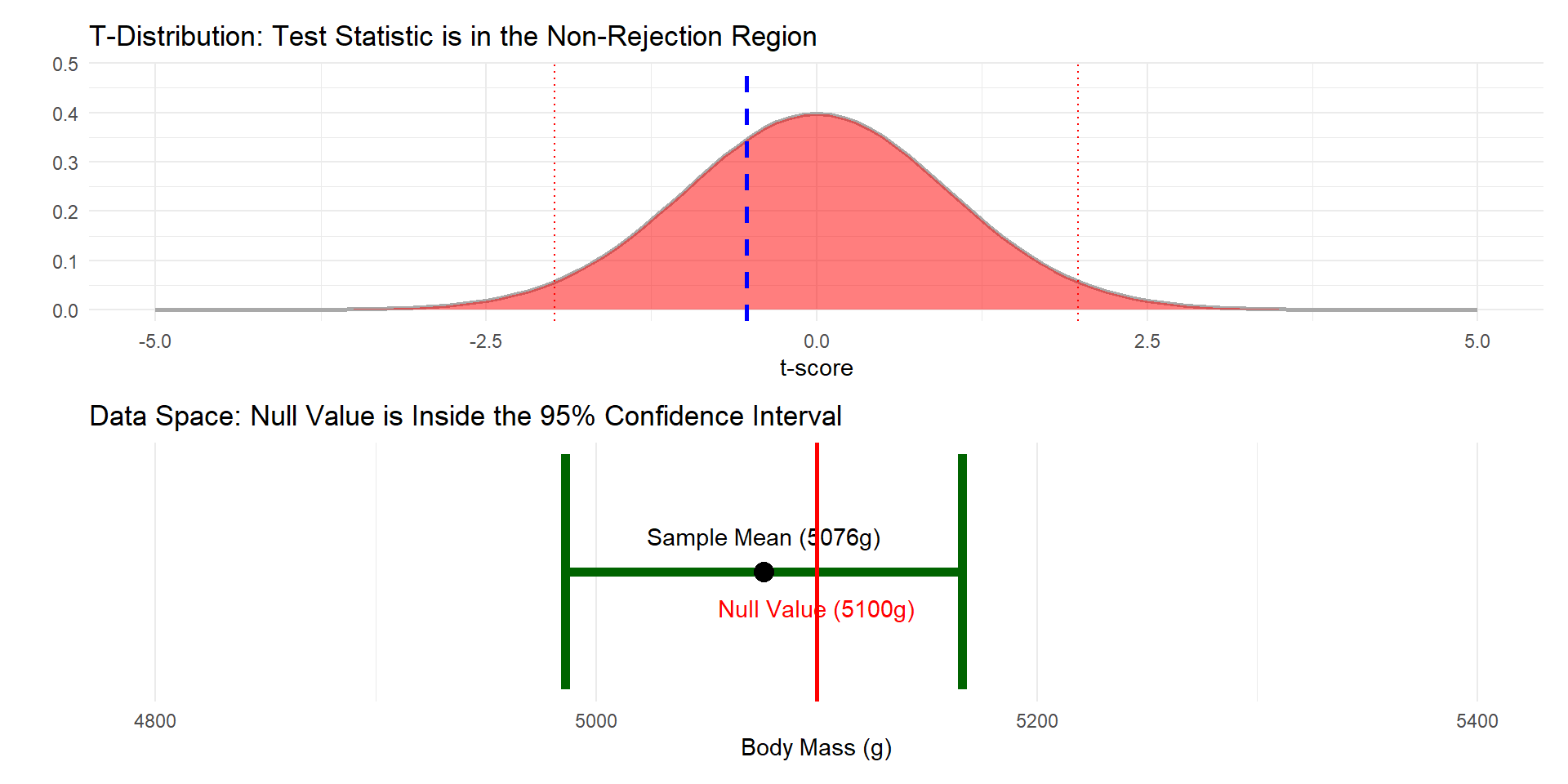
If the hypothesis test leads you to reject the null hypothesis, it means that the distance between \(\bar{x}\) and \(\mu_o\) is greater than the margin of error defined by the 95% CI.