# A tibble: 1 × 2
  mean_bodymass count
          <dbl> <int>
1 5076. 123Single Mean
Dr. Elijah Meyer
NC State University
ST 511 - Fall 2025
2025-10-01
Checklist
– HW-3 due October 5th
– Are you keeping up with the prepare material?
– Quiz (released Thursday due Sunday)
– AE keys are posted
– Homework-3 key will be posted before the exam
We will finish the single_mean repo today. Please clone this if you haven’t!
Exam-1
in-class (October 8th)
– Statistical concepts
– Maybe one coding question
You may bring a hand-written 8x11 note sheet to the exam
Use this for concepts, and equations (ex. SE(\(\hat{p}\)))
Exam-1
take-home (Due October 17th)
– Statistical concepts
– Can you do the stuff we learned in class
Extension Question: Part of being a researcher/statistician is being able to take concepts and apply them in a new setting. There will be an extension question on the exam that will test your critical thinking skills. I will give you the appropriate material with the question to be successful.
Questions?
Last time

Context
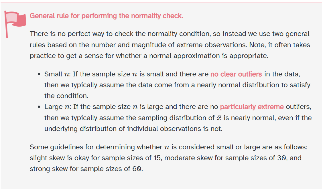
We wanted to look at Penguin’s bodymass for the Gentoo species.
\(H_o: \mu = 6500\)
\(H_a: \mu \neq 6500\)
Assumptions?
# A tibble: 1 × 1
  count
  <int>
1   123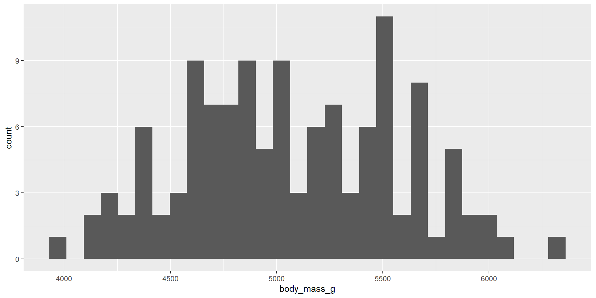
t-test
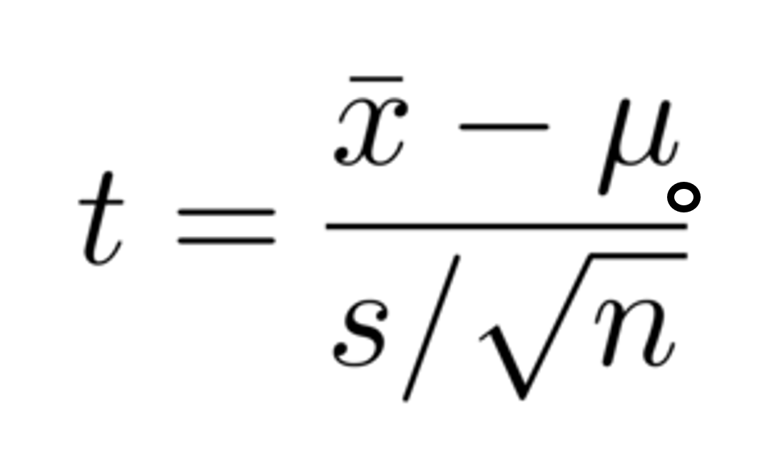
What is:
– A t-distribution
– degrees of freedom?
t-distribution
A t-distribution is similar to a normal distribution, with a little more uncertainty!
– there are infinite t-distributions vs one-normal distribution
– t-distribution approaches a normal distribution when df goes up!
When do we use a t-distribution
We use a t-distribution when the population standard deviation is unknown.
Let’s explain why we used a standard normal for categorical data, and why we will use a t-distribution for quantitative data!
“Linked Together”
For categorical data, our statistic (or assumption in hypothesis testing) is completely linked to the standard error.
We can not change one without the other.
Proportions
\(\hat{p} = \frac{7}{12}\)
\(SE(\hat{p}) = \sqrt{\frac{\frac{7}{12} \left(1 - \frac{7}{12}\right)}{12}} = 0.142\)
\(\hat{p} = \frac{2}{12}\)
\(SE(\hat{p}) = \sqrt{\frac{\frac{2}{12} \left(1 - \frac{2}{12}\right)}{12}} = 0.108\)
When we change the proportion, the standard error changes!
They are “linked together”. When we know one, we have a lot of information about the other.
We use a Z-distribution for hypothesis tests / confidence intervals
Means
n = 5
0,5,10,15,20
\(\bar{x} = \frac{0 + 5 + 10 + 15 + 20}{5} = \frac{50}{5} = 10\)
\(SE_{\bar{x}} = \frac{s}{\sqrt{n}}\)
\(SE_{\bar{x}} = \frac{\sqrt{\frac{\sum_{i=1}^{5} (x_i - 10)^2}{5-1}}}{\sqrt{5}}\)
\(SE_{\bar{x}} = \sqrt{\frac{\frac{250}{4}}{5}} \approx 3.5355\)
Means
n = 5
8,9,10,11,12
\(\bar{x} = \frac{8 + 9 + 10 + 11 + 12}{5} = \frac{50}{5} = 10\)
\(SE_{\bar{x}} = \frac{\sqrt{\frac{\sum_{i=1}^{5} (x_i - 10)^2}{5-1}}}{\sqrt{5}}\)
\(SE_{\bar{x}} = \frac{\sqrt{\frac{10}{5-1}}}{\sqrt{5}} = 0.707\)
Two identical means have entirely different standard error calculations. These are not “linked”, and we need to account for the additional uncertanity by using a t-distribution!
In summary
Why t vs z
– Short answer
  t-distribution for quantitative response
  z-distribution for categorical response
– Long answer
  the sample proportion is linked to the standard error
  the sample mean is not linked to the standard error and the t-distribution accounts for the additional uncertanity in our estimation
t-distribution
there are infinite t-distributions… and their shape depends on the degrees of freedom…
so what are degrees of freedom?
What are degress of freedom?
Degrees of freedom for a t-distribution refer to the number of independent pieces of information that are available to estimate a parameter.
Doc cam example
What are degress of freedom?
If our sample size is 124, our degrees of freedom would be 123.
For example, if you have n = 124, once you know the values of 123 observations, the 124th observation must be whatever makes the math equal \(\bar{x} = 124\)
We have 123 independent pieces of information, and one dependent piece of information.
degrees of freedom
Degrees of freedom are calculated n-1
Note: s is calculated from this constraint on the mean, so degrees of freedom are n-1.
In summary
Degrees of freedom go with t-distributions, and control the shape
For the single mean case, they are calculated to be n-1
This is not necessary for categorical data.
Questions?
single mean ae
If the hypothesis test leads you to reject the null hypothesis, it means that the distance between \(\bar{x}\) and \(\mu_o\) is greater than the margin of error defined by the 95% CI.
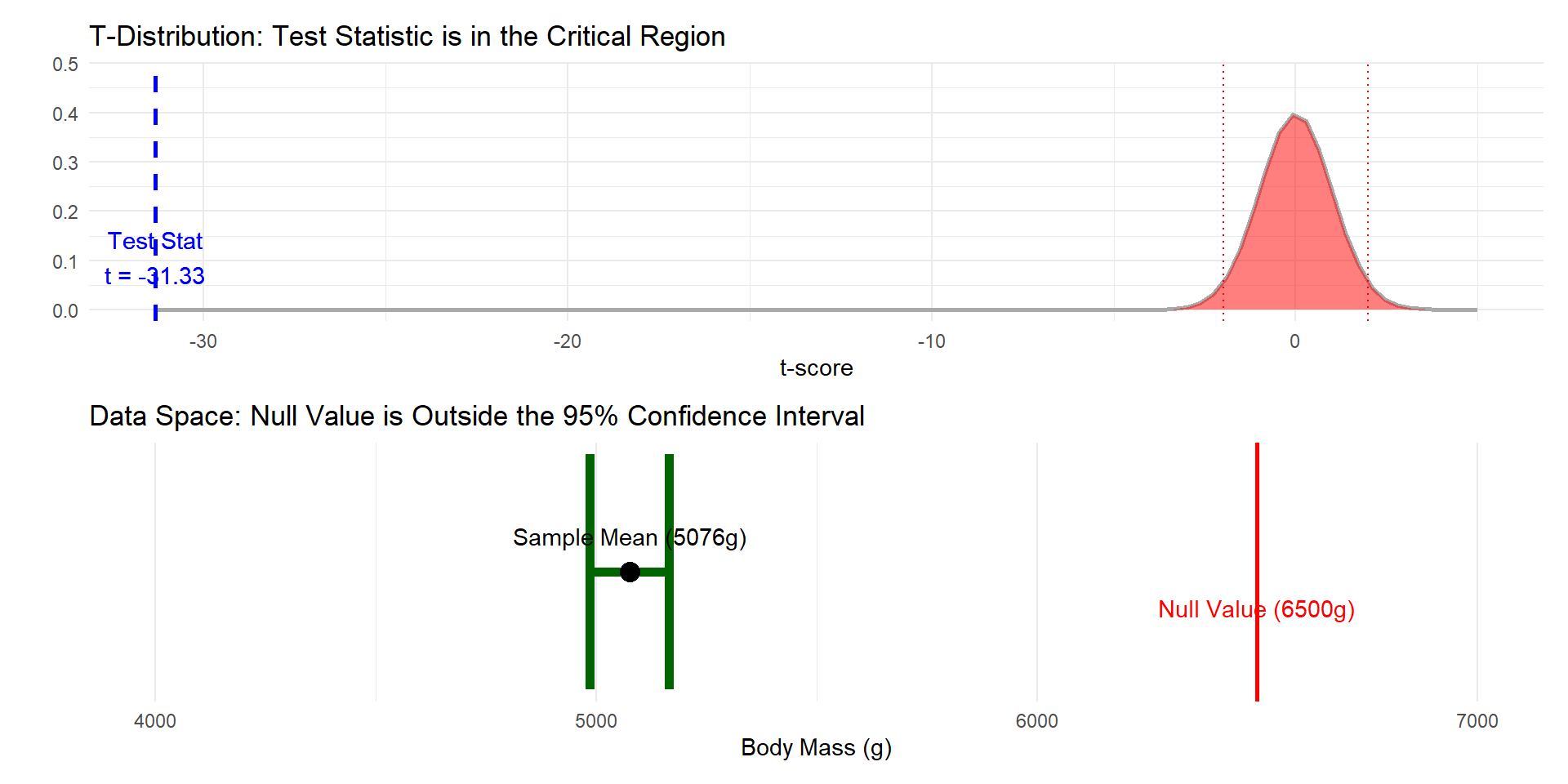
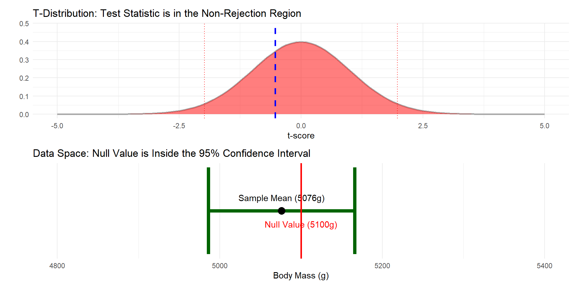
The math
\[ \left| \frac{\bar{x}_1 - \mu_o}{SE} \right| > t^* \]
\[ |\bar{x}_1 - \mu_o| > t^* \times SE \]
This inequality states that the distance from the center of the interval to the null value \(\mu_o\) is greater than the margin of error. If the distance to \(\mu_o\) is longer than the margin of error around the sample mean, the confidence interval must exclude \(\mu_o\).
More notes
These two equations are mathematically equivalent, proving that rejecting \(H_o\) is the same as the confidence interval excluding the null value \(\mu_o\).
– For a two-sided test where \(\alpha\) “matches up” with our confidence level
ex. \(\alpha\) = 0.05 and a 95% confidence interval
For categorical data
The difference in their numerical values is usually too small to break the equivalence.