| term | estimate | std.error | statistic | p.value |
|---|---|---|---|---|
| (Intercept) | 147.951 | 4.174 | 35.447 | 0 |
| bill_length_mm | 1.083 | 0.107 | 10.129 | 0 |
| speciesChinstrap | -5.004 | 1.370 | -3.653 | 0 |
| speciesGentoo | 17.799 | 1.170 | 15.216 | 0 |
Multiple Linear Regression
Dr. Elijah Meyer
NC State University
ST 511 - Fall 2025
2025-11-10
Checklist
– Quiz released Wednesday (due Sunday)
– Homework has been assigned (due Sunday)
– Statistics experience released
– Final Exam is Dec 8th at 3:30 (expect an email this afternoon)
What’s left
Homework 35% (1 or 2 more)
Quizzes 15% (1 or 2 more)
Statistics Experience 5% (due last day of class)
Exam 01 (in-class) 12.5%
Exam 01 (take home) 12.5%
Final Exam 20% (December 8th)
Regrades
Open Monday through Friday
We know the drill
Last Time
We learned simple linear regression.
What is it?
Simple linear regression
Population level: \(y = \beta_o + \beta_1*x + \epsilon\)
Sample: \(\hat{y} = \hat{\beta_o} + \hat{\beta_1}*x\)
Hypothesis Testing
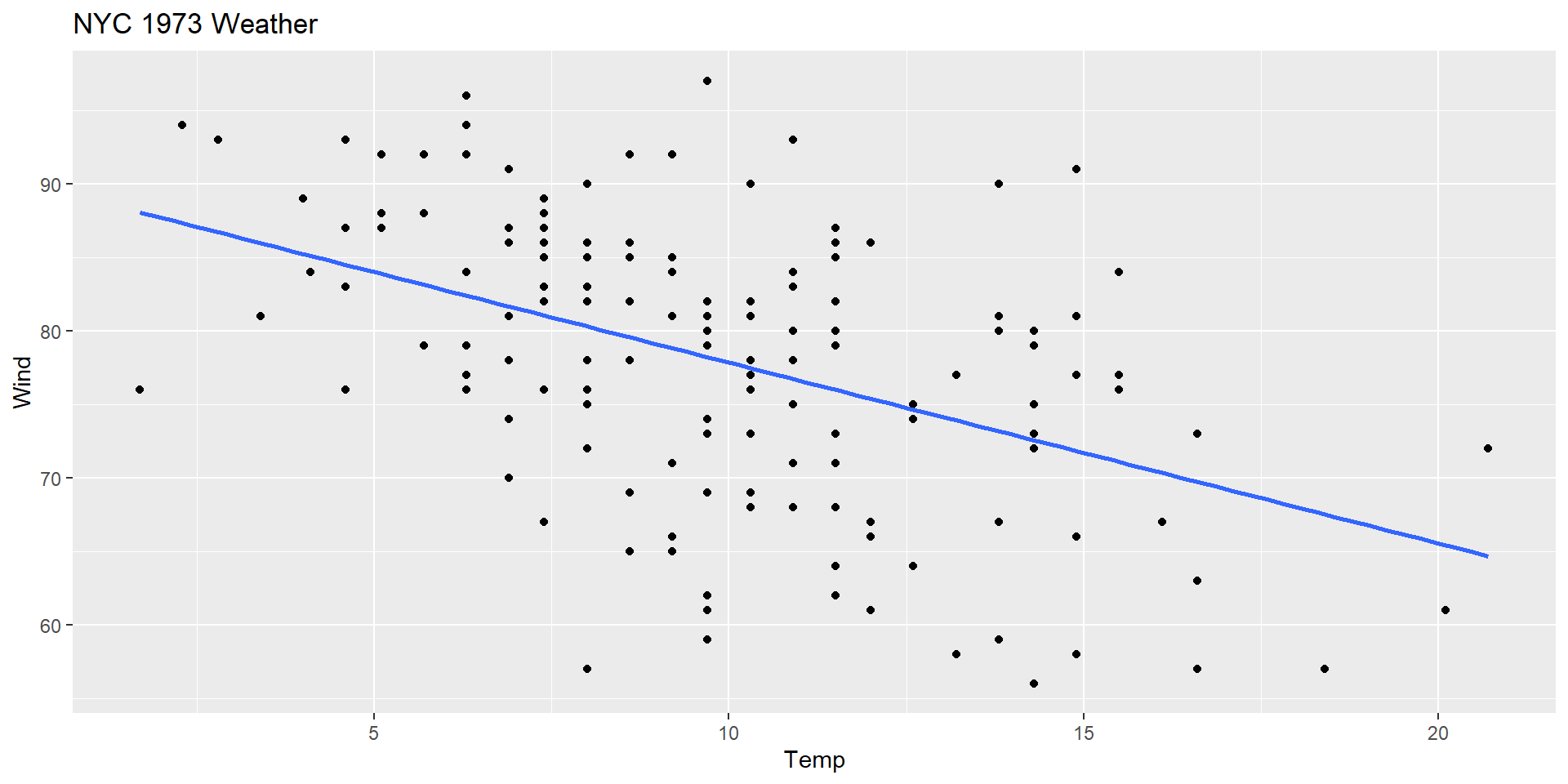
… and if I want to test for a linear relationship between Temp and Wind at the population level, what’s the proper notation?
Null and alternative
\(H_o: \beta_1\) = 0
\(H_a: \beta_1 \neq 0\)
Assumptions?
Assumptions
– Independence (how we sample)
– Linear relationship (scatterplot / residual vs fitted)
– Equal Variance (residual vs fitted)
– Normality or residuals (normal q-q plot)
plot(model) will get you these plots!
test statistic?
test-statistic
\[t = \frac{\hat{\beta}_1 - \beta_{\text{null}}}{\text{SE}(\hat{\beta}_1)}\]
And this t-statistic follows a t-distribution with n-2 degrees of freedom (-2 because we estimate the population slope and intercept)
Other models
Goals for today
– Understand multiple linear regression
– additive vs interaction
… next class, we will do hypothesis testing
Multiple Linear Regression
Sometimes, you need a more complicated model to help best understand the variability in your response variable.
Multiple linear regression
– Quantitative response (Y)
– > 1 explanatory variable
Penguins
Things to note
– The values of the coefficients change when we add more variables into our model
– We are going to demonstrate multiple linear regression with 1 categorical explanatory variable and 1 quantitative explanatory variable… but it doesn’t need to be this way! For example, we can have two quantitative explanatory variables.
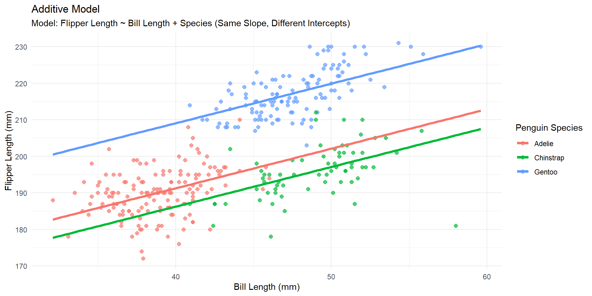
Additive model
The relationship between x and y does not depend on z
Model Output
General Formula
\[ \hat{Y} = \hat{\beta}_0 + \hat{\beta}_1 X_1 + \hat{\beta}_2 X_2 + \dots + \hat{\beta}_k X_k \]
Simple linear regression
| term | estimate | std.error | statistic | p.value |
|---|---|---|---|---|
| (Intercept) | 126.684 | 4.665 | 27.156 | 0 |
| bill_length_mm | 1.690 | 0.105 | 16.034 | 0 |
Multiple linear regression (additive)
| term | estimate | std.error | statistic | p.value |
|---|---|---|---|---|
| (Intercept) | 147.951 | 4.174 | 35.447 | 0 |
| bill_length_mm | 1.083 | 0.107 | 10.129 | 0 |
| speciesChinstrap | -5.004 | 1.370 | -3.653 | 0 |
| speciesGentoo | 17.799 | 1.170 | 15.216 | 0 |
Let’s write the full equation out.
Now, let’s write out the equation for each of the three individual species!
Interpretation
How do we interpret 1.083?
How do we interpret 17.799?
Interpretations
Holding species constant, for a 1 mm increase in bill length, we estimate an average increase in flipper length of 1.083mm.
Holding bill length constant, we estimate the mean flipper length of Gentoo penguins to be 17.799mm larger than the Adelie penguins.
In R
Additive model
Reminder: With two quantitative explanatory variables!
Questions?
Multiple linear regression (interaction)
Assumption:
The relationship between x and y depends on the values of z
Interaction model
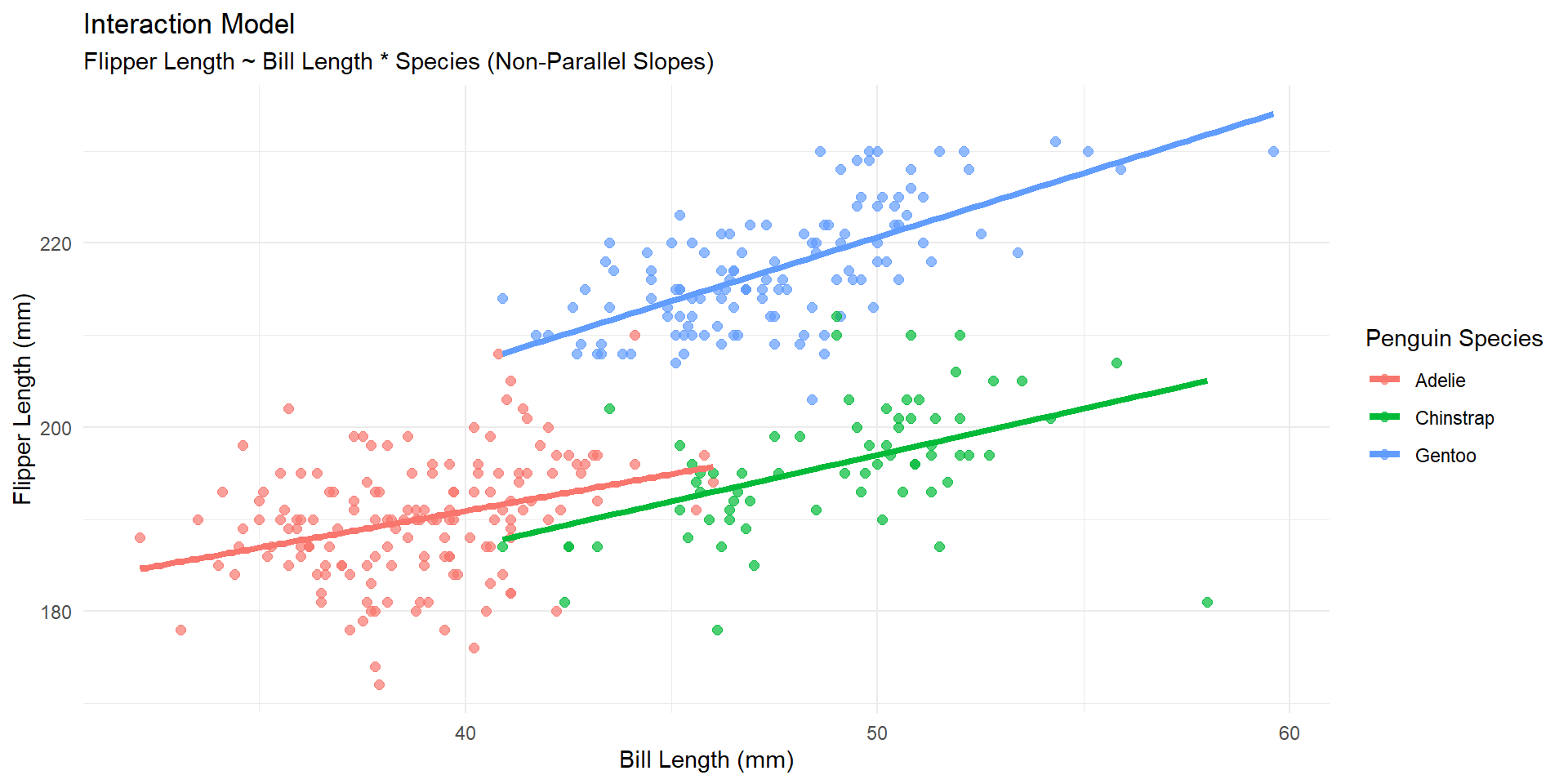
Output
# A tibble: 6 × 5
  term                            estimate std.error statistic  p.value
  <chr>                              <dbl>     <dbl>     <dbl>    <dbl>
1 (Intercept)                      159.        6.90     23.0   4.72e-71
2 bill_length_mm                     0.800     0.178     4.50  9.17e- 6
3 speciesChinstrap                 -12.3      12.5      -0.986 3.25e- 1
4 speciesGentoo                     -7.83     10.6      -0.736 4.63e- 1
5 bill_length_mm:speciesChinstrap    0.207     0.276     0.750 4.54e- 1
6 bill_length_mm:speciesGentoo       0.591     0.246     2.40  1.67e- 2
How do we interpret 0.207?
Interpretation
For a 1 mm increase in bill length, we estimate an average increase in flipper length of 0.207mm more for Chinstrap than Adelie penguins, holding all OTHER variables constant
Ex. Holding Gentoo constant at 0.