Logistic Regression
Lecture: 4th to last!
NC State University
ST 511 - Fall 2025
2025-11-17
Checklist
– HW 6 released Wednesday (our last HW!)
– Quiz 11 (released Wednesday; due Sunday)
– Don’t forget about the statistics experience
– Final Exam is Dec 8th at 3:30
– We DO have an AE today. Please clone this and have it ready for class.
Warm Up
Why are we learning all of this?
Statistical Inference vs Sampling Variability
Statistical Inference - taking a sample, and making claims about a larger population
Sampling variability - the natural variability (error) we expect/see from sample to sample
Sampling Variability
Let’s assume that Gen-Z has a mean credit score of 680 (\(\mu = 680\)). If you take a random sample of 100 Gen-Z individuals, would we expect the mean credit score of those 100 to be exactly 680?
Inference
Because we know this, we account for sampling variability by using distributions (instead of just point estimates) when trying to make claims about an entire population!
What type of question would we not need statistical inference for?
Examples
– In ST 312 for the Fall 2025 semester, are the average grades in Teacher A’s class higher than Teacher B’s class?
– Is the weather today different than the weather tomorrow?
Summary
You are researchers that ask questions (typically) at the population level, to:
– learn more
– make data driven decisions
– etc.
Because we know sampling variability exsists, we can’t make sweeping claims by comparing point estimates without some understanding of variability.
Questions
Scenarios
It’s important for us to know when methods are vs are not appropriate, based on variable type. We are going to go through three examples and identify each scenario on which methods would be most appropriate to answer the research question.
Example 1
An ecologist is studying a population of small mammals (e.g., field mice) to see if their primary habitat is associated with their dominant predator avoidance tactic.
| Hiding/Freezing | Fleeing/Running | Row Totals | |
|---|---|---|---|
| Forest | 80 | 20 | 100 |
| Scrubland | 45 | 55 | 100 |
| Open Field | 15 | 85 | 100 |
| Column Totals | 140 | 160 | N = 300 |
Example 2
What was the median student loan debt for all 350 students who graduated from the Engineering School in May 2025?
Example 3
A pharmacologist is studying the factors that influence patient Recovery Time (in days) following a specific surgical procedure. They are analyzing the effects of a new post-operative drug and the patient’s age.
The researcher hypothesizes a significant interaction between the two factors: the new drug may be highly effective (significantly reducing recovery time) for younger patients, but its efficacy might be greatly reduced or even disappear for older patients due to metabolic changes.
Questions?
New material
Goal
Gain some exposure to logistic regression
We can’t learn everything in a week, but we can start to build a foundation
Goal
– The What, Why, and How of Logistic Regression
– How to fit these types of models in R
– How to calculate probabilities using these models
What is Logistic Regreesion
Similar to linear regression…. but
Modeling tool when our response is categorical
AE for motivation
The problem
(\(\mu_y\)) = (\(\beta_0 + \beta_1 X_1 + \dots\))
The right side of a regression equation, which can take any value from \(-\infty\) to \(+\infty\).
(\(\mu\)): The expected value of the response variable, which is restricted to a certain range (e.g., a probability must be between 0 and 1).
The solution
Applying a specific mathematical transformation to the expected outcome (or mean) of your model in order to linearly relate it to your predictor variables, while restricting the values of your response variable accordingly.
For logistic regression, this is the the logit-link function!
(\(\mu_y\) or \(p\))
\(ln(\frac{p}{1-p})\)
\(\widehat{ln(\frac{p}{1-p}})\) = \(\widehat{\beta_o} +\widehat{\beta}_1X1 + ....\)
What we will do today
– This type of model is called a generalized linear model
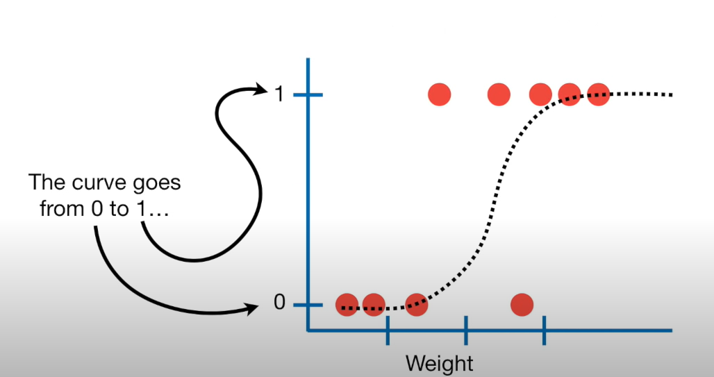
We want to fit an S curve (and not a straight line)…
where we model the probability of success as a function of explanatory a variable(s)
Terms
– Bernoulli Distribution
2 outcomes: Success (p) or Failure (1-p)
\(y_i\) ~ Bern(p)
Note: We use \(p_i\) for estimated probabilities
The model
\(\widehat{ln(\frac{p}{1-p}})\) = \(\widehat{\beta_o} +\widehat{\beta}_1X1 + ....\)
Breaking down the model
\(ln(\frac{p}{1-p})\) is called the logit link function, and can take on the values from \(-\infty\) to \(\infty\)
\(ln(\frac{p}{1-p})\) represents the log odds of a success
log odds
\(ln(\frac{p}{1-p})\) = natural logarithm of the odds, where the odds are the ratio of the probability of an event happening to the probability of it not happening
\(ln(\frac{p}{1-p})\) has good modeling properties (ex. unbounded; handles extreme values of p well for linearity; restricts p to be between 0 and 1)… but the interpretation is tough (not very useful?)
Think of this as our initial model, that we will work with to model probabilities (can also model odds)
Probability
p stands for probability
This logit link function restricts p to be between the values of [0,1]
Which is exactly what we want!
Let’s show this!
Math
We want to model probabilities. We want to isolate p on the left side of this equation.
\(\widehat{ln(\frac{p}{1-p}})\) = \(\widehat{\beta_o} +\widehat{\beta}_1X1 + ....\)
How do we isolate p? That is, how to we get rid of the ln?
So
\[\widehat{ln(\frac{p}{1-p}}) = \widehat{\beta_o} +\widehat{\beta}_1X1 + ....\]
– Lets take the inverse of the logit function
– Demo Together
Final Model
\[\hat{p} = \frac{e^{\widehat{\beta_o} + \widehat{\beta_1}X1 + ...}}{1 + e^{\widehat{\beta_o} + \widehat{\beta_1}X1 + ...}}\]
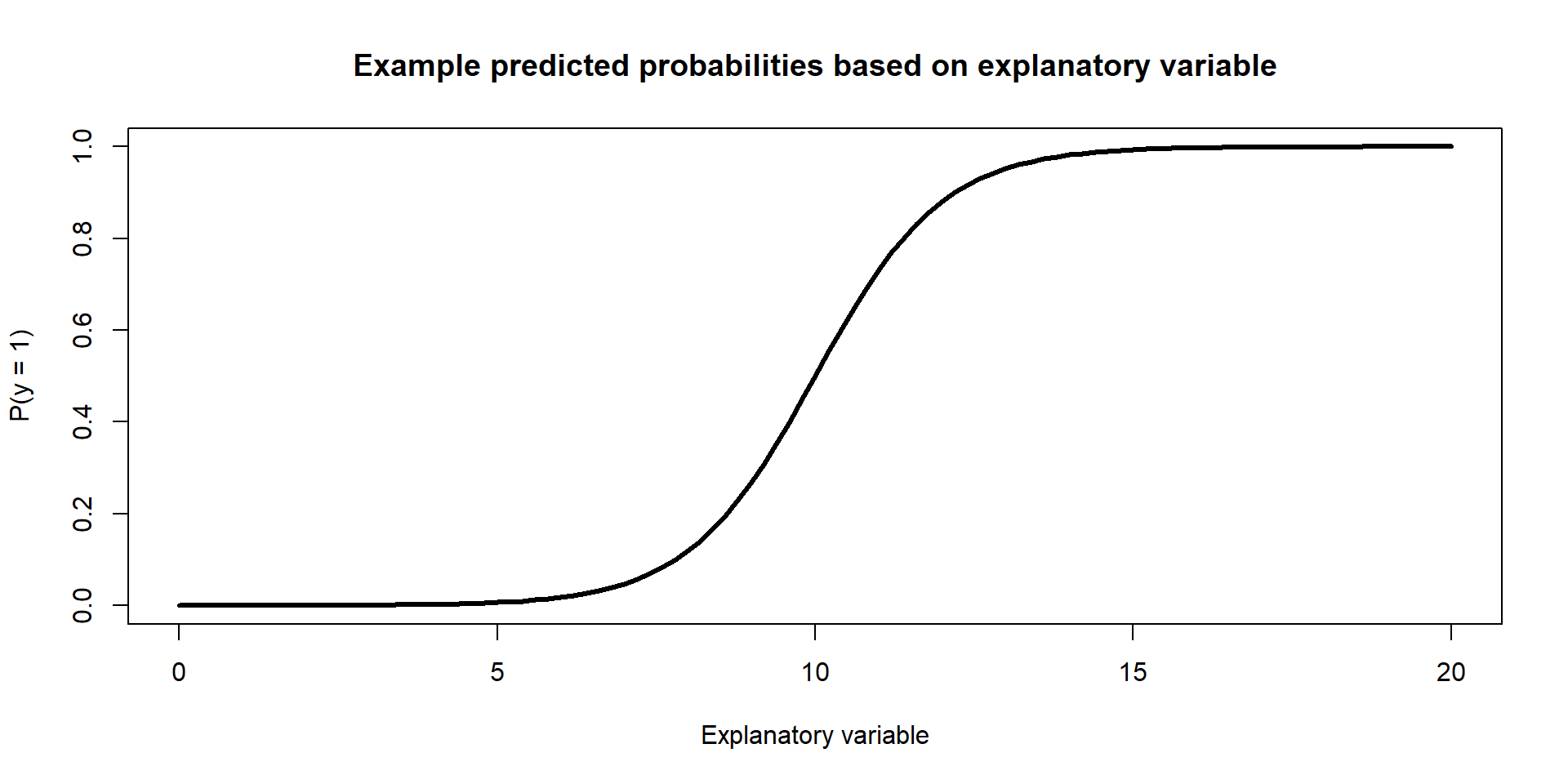
Example Figure:
Recap
With a categorical response variable, we use the logit link (logistic function) to calculate the log odds of a success
\(\widehat{ln(\frac{p}{1-p})}\) = \(\widehat{\beta_o} +\widehat{\beta}_1X1 + ....\)
We can use the same model to estimate the probability of a success
\[\hat{p} = \frac{e^{\widehat{\beta_o} + \widehat{\beta_1}X1 + ...}}{1 + e^{\widehat{\beta_o} + \widehat{\beta_1}X1 + ...}}\]
AE
Takeaways
– We can not model these data using the tools we currently have
– We can overcome some of the shortcoming of regression by fitting a generalized linear regression model
– We can model binary data using an inverse logit function to model probabilities of success