The meaning of confidence is about what happens in the long-run!
If we make many many confidence intervals under the same circumstances, we would expect ____% to actually capture the true parameter of interest!
Warm-up
How is this different than interpreting our single calculated confidence interval?
Last time, we calculated a 95% confidence interval in our Howling Cow exercise to be:
(0.276, 0.464)
Interpret this confidence interval in the context of the problem.
Interpretation
We are 95% confident that the true proportion of students who eat Howling Cow ice creme at NC State is between 0.276 and 0.464.
Calculate a __% confidence interval
\(\hat{p} \pm z^* * SE(\hat{p})\)
.37 \(\pm\) 1.96*0.0482
.37 \(\pm\) 0.094
.37 + 0.094 = 0.464
.37 - 0.094 = 0.276
(0.276, 0.464)
Practice
Instead, calculate a 90% confidence interval. Now calculate an 80% confidence interval. What changes? Why might we choose a specific confidence level?
Confidence intervals
qnorm(.95)
[1] 1.644854
.37 \(\pm\) 1.645*0.0482 = (0.291, 0.49)
qnorm(.90)
[1] 1.281552
.37 \(\pm\) 1.28*0.0482 = (0.308, 0.432)
Questions?
Difference in proportions
What happens when we work with two variables?
– What’s the same?
– What’s different?
Example
A pharmaceutical company is conducting a clinical trial to test the effectiveness of a new drug for a common illness. They randomly assign participants to one of two groups
Group 1 (New Drug): Out of 200 patients, 160 recovered from the illness.
Group 2 (Placebo): Out of 180 patients, 126 recovered from the illness.
Perform a hypothesis test to determine if the proportion of patients who recovered is significantly different for the group that received the new drug
– What’s our variable(s)?
– Null and alternative hypothesis?
– Statistic?
Take-aways
– Our population parameter gets more complicated!
– Order matters!
– Our null hypothesis (nothing weird is going on) can be thought of as the “groups don’t matter”.
Pharmaceutical Example
\(H_o: \pi_n - \pi_p = 0\)
\(H_o: \pi_n - \pi_p > 0\)
\(\hat{p_n} - \hat{p_p} = .1\)
What assumptions did we have to check last time in order to do a hypothesis test?
Assumptions
– Independence (observation level, not variables)
– Success-failure (sample size)
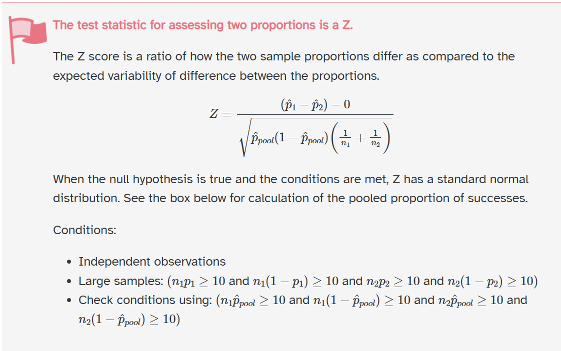
Sucecss-failure
\(p_\text{pool} * n1\) > 10?
\((1- p_\text{pool}) * n1\) > 10?
\(p_\text{pool} * n2\) > 10?
\((1- p_\text{pool}) * n2\) > 10?
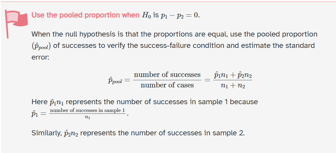
p-pooled
\(\frac{168 + 126}{200 + 180}\) = .774
\(.774 * 200\) > 10?
\(.226 * 200\) > 10?
\(.774 * 180\) > 10?
\(.226* 180\) > 10?
Let’s do a hypothesis test!
Z-test
Because it’s common to standardize, we will perform a z-test.
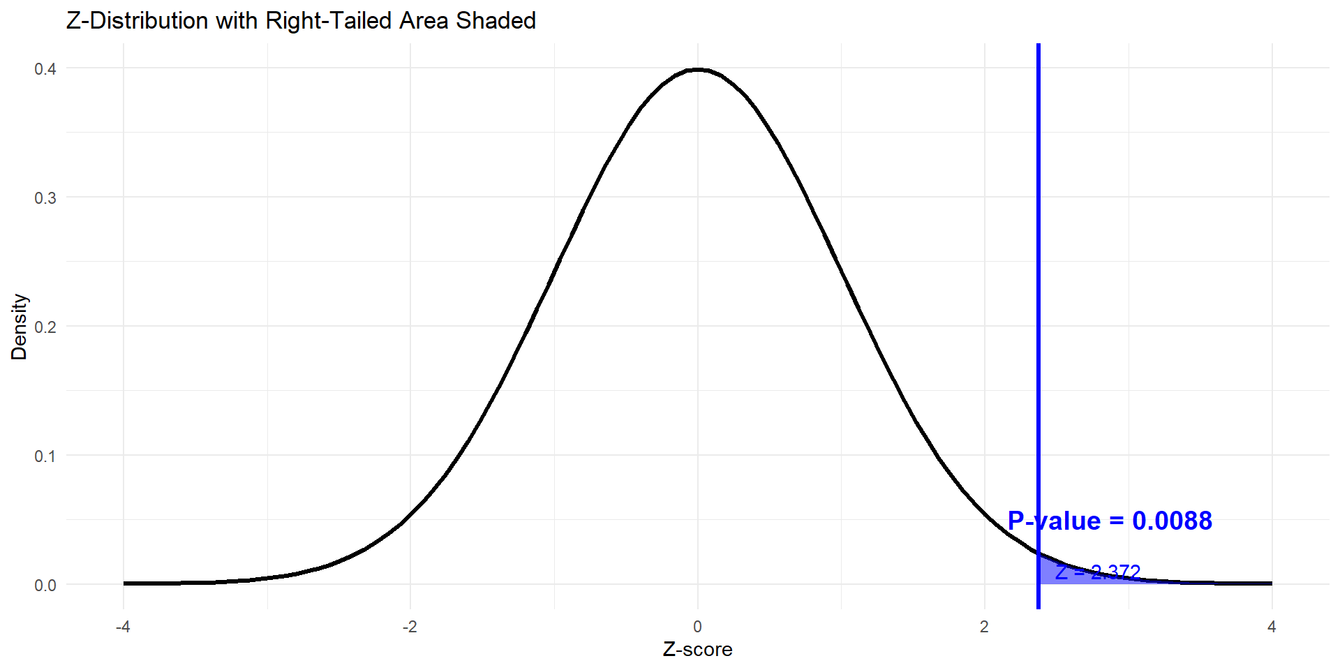
On a piece of paper, draw what this would look like, and shade in the area of the p-value.
What does it look like
The p-value for Z = 2.372 is: 0.0088
Confirm the p-value from the graph.
Next, write a decision and conclusion at the \(\alpha\) = 0.05 in the context of the problem.
Decission and Conclusion
Because or p-value is < \(\alpha\), we reject the null hypothesis, and have strong evidence to conclude that the true proportion of patients who recovered from the illness taking the new drug is larger than those who took the placebo.
Let’s estimate it!
Confidence intervals and hypothesis testing
Typically, you report both in research.
Let’s estimate what \(\pi_n - \pi_p\) actually is!
Assumptions
Independence (check)
Success-failure (how is this different than hypothesis testing?)
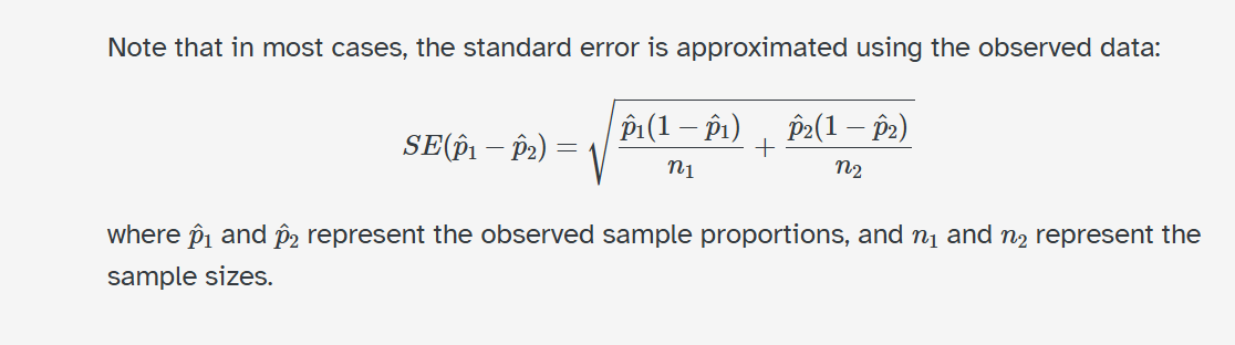
Now, let’s use our best guess for \(\pi_n - \pi_p\) with our estimated standard error to approximate the sampling distribution!
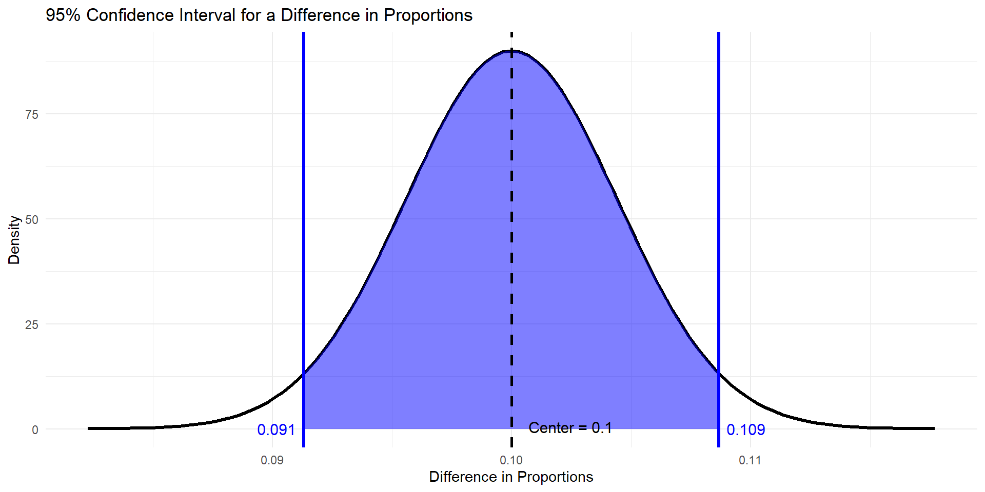
Plot
\(.1 + .00443 * 1.96\)
\(.1 - .00443 * 1.96\)
Interpret
We are 95% confident that the true proportion of patients who took the new drug and recovered is 0.091 to 0.109 HIGHER than the true proportion of patients who took the placebo and recovered.
New things:
– Direction!
Questions
Next time
Relationship between the two
When you are working with a two-tailed test…
If you reject the null hypothesis at the \(\alpha = 0.05\) level, then we would expect our 95% confidence interval to NOT include the null value!
The condition for rejecting the null hypothesis is that the absolute Z-statistic is greater than the critical value \(|Z_{stat}| > Z_{crit}\).
We can rearrange the inequality above to show: \(|\hat{p} - p_0| > Z_{crit}\sqrt{\frac{\hat{p}(1-\hat{p})}{n}}\)
Quantitative variables
The key insight is that when you reject the null hypothesis, the distance between your statistic and the null value is larger than the margin of error of the confidence interval. Since the null value is a certain distance away from your sample proportion, and that distance is greater than the width of your confidence interval, the null value cannot possibly be inside the interval.