# A tibble: 6 × 3
# Groups:   species [3]
  species   sex    count
  <fct>     <fct>  <int>
1 Adelie    female    73
2 Adelie    male      73
3 Chinstrap female    34
4 Chinstrap male      34
5 Gentoo    female    58
6 Gentoo male 61Finish One-way Anova
& Chi-Square
Dr. Elijah Meyer
NC State University
ST 511 - Fall 2025
2025-10-26
Checklist
– I’m grading your take-homes now
– Quiz released Wednesday (due Sunday)
– Homework released last Friday (due this Friday)
– Statistics experience released
– Final Exam is Dec 8th at 3:30
Last Time
We were looking at bill length across all three species of Penguin. Open up the anova-cor R-Project. We are going to finish this activity.
Penguins
New question
Suppose that we want to look at the relationship between sex and species. That is, we want to test if species of penguin is independent from sex. How is this different than what we’ve done before?
Type of test
Can we use difference in means?
Difference in proportions?
Chi-square test
The big picture idea is to compare expected counts (under the assumption of the null hypothesis with observed counts. This is how we are going to calculate our test statistic.
Chi-square test
\(Ho:\)
\(Ha:\)
Chi-square test
\(Ho: \text{sex and species of penguins are independent}\)
\(Ha: \text{sex and species of penguins are not independent}\)
Steps of a null hypothesis
– Set up the null and alternative hypotheses
– Collect data
– Check assumptions (so we can trust our theory based tests)
– Calculate our test statistic
– p-value
– decisions and conclusions
Table
What would we expect to see under the assumption of the null hypothesis?
What did we actually observe?
Are the differences “statistically significant”?
| Male | Female | Total | |
|---|---|---|---|
| Adelie | 146 | ||
| Chinstrap | 68 | ||
| Gentoo | 119 | ||
| Total | 168 | 165 | 333 |
Assumptions
– Independence
– Expected frequencies (sample size condition)
Expected frequencies
Your book says that each expected cell count should be > 5. This will be our rule of thumb.
If any of the expected values are low the p-values generated by the test start to become less reliable.
We will check this when we make a table!
Under the hood
Binomial Approximation: The observed counts in a contingency table follow a binomial distribution
The CLT tells us that when the number of trials (\(n\)) is large enough, the binomial distribution can be reasonably approximated by the normal distribution
The Chi-Square test relies on the assumption that the sampling distribution of the observed frequencies (counts) is close enough to a normal distribution for the \(\chi^2\) statistic to accurately follow the theoretical Chi-Square distribution.
When Expected Counts are High (≥5): The underlying discrete (integer) count data behaves smoothly, like a continuous, bell-shaped (Normal) curve (CLT).
When Expected Counts are Low (<5): The data distribution remains highly skewed and chunky (discrete). It looks nothing like the smooth Normal distribution.
What you need to be able to articulate
If our sample size assumption (expected counts) is not met, the test statistic doesn’t actually follow the distribution it’s being compared to…. so we can’t trust the results.
Chi-square test
The big picture idea is to compare expected counts (under the assumption of the null hypothesis with observed counts. This is how we are going to calculate our test statistic.
Null hypothesis (reminder)
\(Ho\) Species has no impact on sex OR Species is completely independent from sex
\(Ha\) Species has some impact on sex OR Species is not independent from sex
Chi-square test
The big picture idea is to compare expected counts (under the assumption of the null hypothesis with observed counts. This is how we are going to calculate our test statistic.
– Null hypothesis ✔️
Expected counts
Expected counts
With a sample size of 333, what would we expect to see in this table under the assumption that species and sex are independent?
Table of EXPECTED counts
| Male | Female | Total | |
|---|---|---|---|
| Adelie | 146 | ||
| Chinstrap | 68 | ||
| Gentoo | 119 | ||
| Total | 168 | 165 | 333 |
Expected Formula
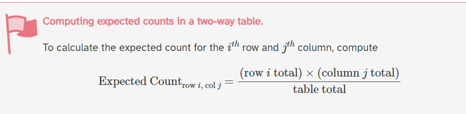
Expected counts
With a sample size of 333, what would we expect to see in this table under the assumption that species and sex are independent?
Pick one cell, and calculate the expected count!
Table of EXPECTED counts
| Male | Female | Total | |
|---|---|---|---|
| Adelie | 146 | ||
| Chinstrap | 68 | ||
| Gentoo | 119 | ||
| Total | 168 | 165 | 333 |
Expected Table
| Male | Female | Total | |
|---|---|---|---|
| Adelie | (146*168)/333 | 146 | |
| Chinstrap | (68*168)/333 | 68 | |
| Gentoo | (119*168)/333 | 119 | |
| Total | 168 | 165 | 333 |
Expected Table
| Male | Female | Total | |
|---|---|---|---|
| Adelie | 73.658 | 146 | |
| Chinstrap | 34.306 | 68 | |
| Gentoo | 60.036 | 119 | |
| Total | 168 | 165 | 333 |
If there is no difference between sex and species, we would expect to observe this values above from our sample.
Expected Table
| Male | Female | Total | |
|---|---|---|---|
| Adelie | 73.658 | (146*165)/333 = 72.343 | 146 |
| Chinstrap | 34.306 | (68*165)/333 = 33.694 | 68 |
| Gentoo | 60.036 | (119*165)/333 = 58.964 | 119 |
| Total | 168 | 165 | 333 |
Are these all larger than 5?
Chi-square test
The big picture idea is to compare expected counts (under the assumption of the null hypothesis with observed counts. This is how we are going to calculate our test statistic.
– Null hypothesis ✔️
– Expected ✔️
– Observed counts
Observed
| Male | Female | Total | |
|---|---|---|---|
| Adelie | 73 | 73 | 147 |
| Chinstrap | 34 | 34 | 68 |
| Gentoo | 61 | 58 | 119 |
| Total | 168 | 165 | 333 |
Observed vs Expected
Expected values are in ( )
| Male | Female | Total | |
|---|---|---|---|
| Adelie | 73 (73.658) | 73 (72.342) | 146 |
| Chinstrap | 34 (34.306) | 34 (33.694) | 68 |
| Gentoo | 61 (60.036) | 58 (58.964) | 119 |
| Total | 168 | 165 | 333 |
What do we think? Without doing a formal test, do you think we will reject or fail to reject the null hypothesis? Why?
Chi-square test
The big picture idea is to compare expected counts (under the assumption of the null hypothesis with observed counts. This is how we are going to calculate our test statistic.
– Null hypothesis ✔️
– Expected ✔️
– Observed counts ✔️
Let’s perform the test
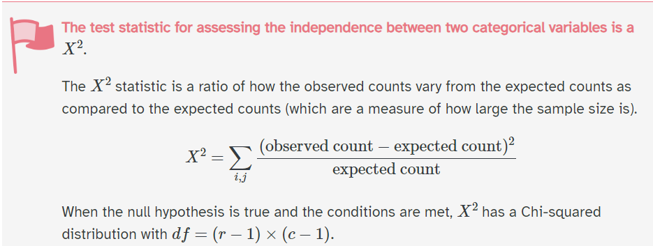
where r is the number of groups for one variable (rows) and c is the number of groups for the second variable (columns)
Chi-sqaure
– The shape of the chi-square distribution curve depends on the degrees of freedom
– Test statistic can not be negative
– The chi-square distribution curve is skewed to the right, and the chi-square test is always right-tailed
– A chi-square test cannot have a directional hypothesis. A chi-square value can only indicate that a relationship exists between two variables, not what the relationship is.
Questions
Calculating a p-value
You can use a table.
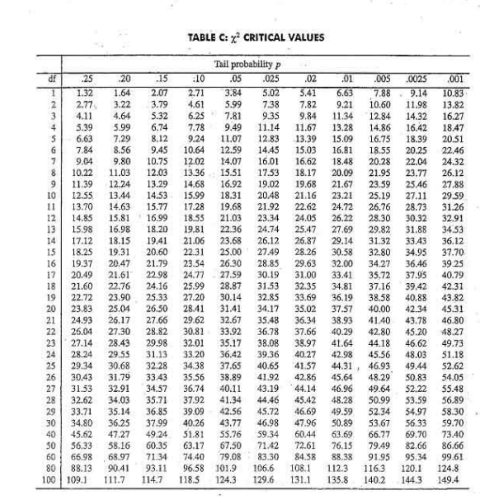
Calculating a p-value
We can use software.
Proper notation
P(\(\chi^2 \geq X^2\)) = p-value
The probability of observing our statistic, or something larger given the null hypothesis is true.
\(\chi^2\) = map of possible outcomes on the chi-sq distribution (random variable because it is generated from a random process)
\(X^2\) = your statistic calculated
Let’s talk about it
Decision?
Conclusion?
Let’s talk about it
Fail to reject the null hypothesis
Weak evidence to conclude that species has an impact on sex
Summary
– Chi-square testing is used when we want to test for independence when we have a categorical variable with > 2 levels
– Always right tailed test
– df of (r-1)*(c-1)