# A tibble: 3 × 3
group count mean
<fct> <int> <dbl>
1 ctrl 10 5.03
2 trt1 10 4.66
3 trt2 10 5.53One-way Anova
Dr. Elijah Meyer
NC State University
ST 511 - Fall 2025
2025-10-20
Checklist
– Exam-1 (in-class) is posted
  > Solutions on Moodle
  > Regrade requests open Wednesday (until Sunday)
– I’m grading your take-homes now
– Quiz released Wednesday (due Sunday)
– Homework released Friday (due next Friday)
– Statistics experience released
Regrades
– This is not a place to spam regrades for points back
– I will regrade your question. The points may go up. The points may go down.
Final notes
Hard work is really clear. Thank you for that.
If you would like to make an appointment to go over the material, please let Nick/I know.
Next exam is the final exam.
Questions
Last Time
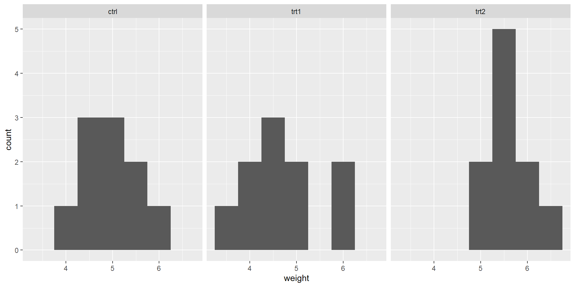
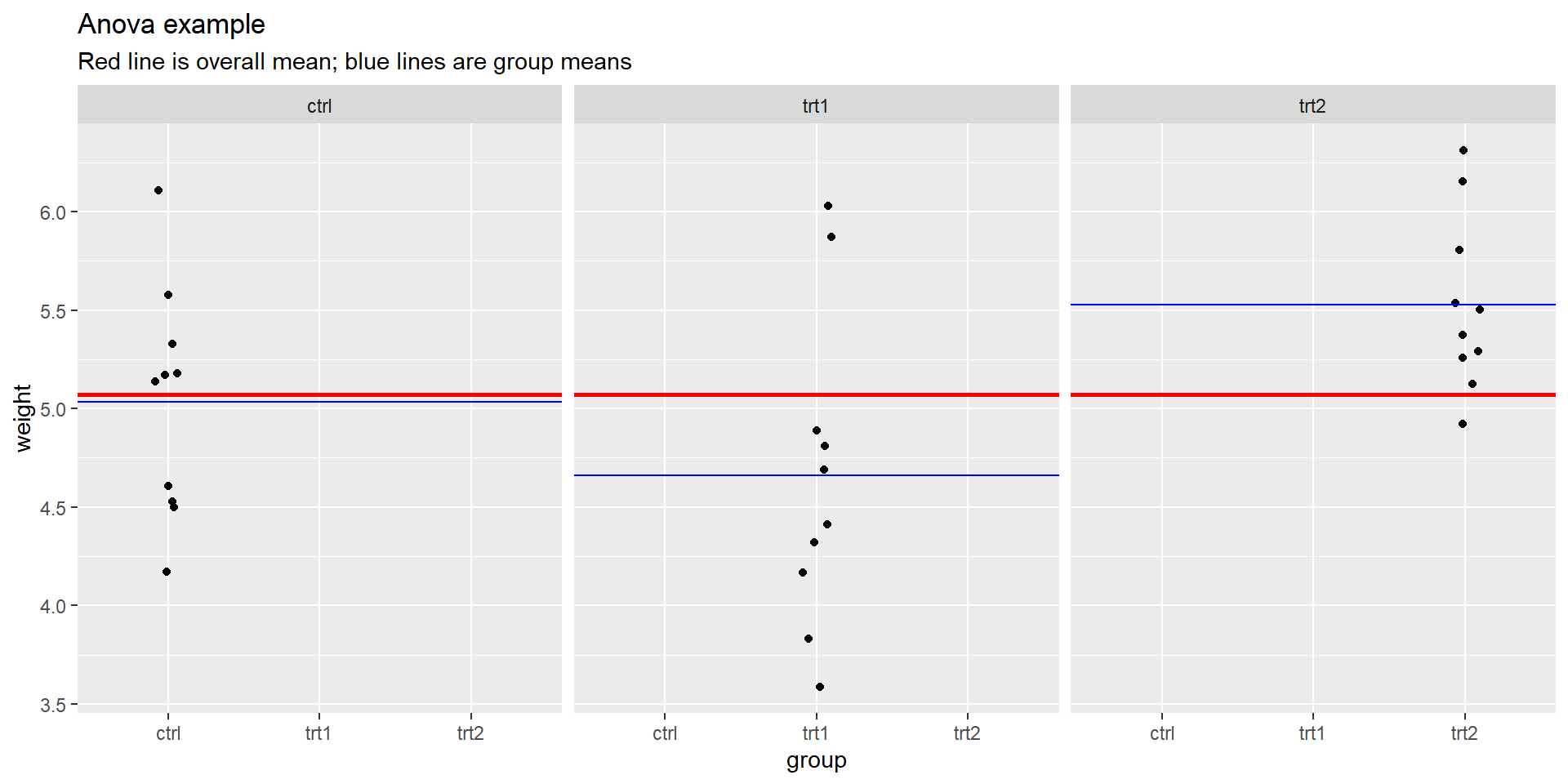
Results from an experiment to compare yields (as measured by dried weight of plants) obtained under a control and two different treatment conditions.
Why can we not answer this question using difference in means?
Extension
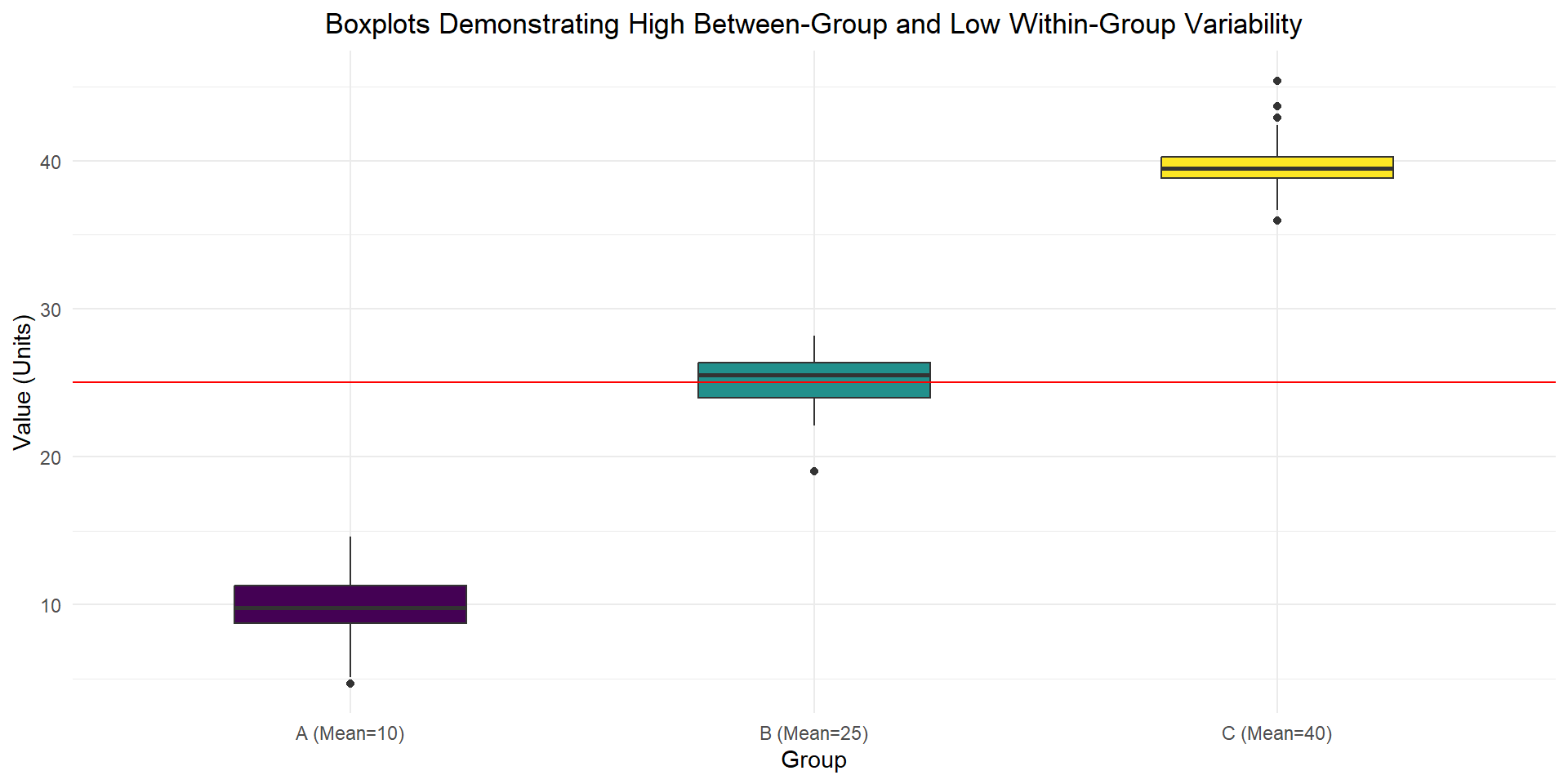
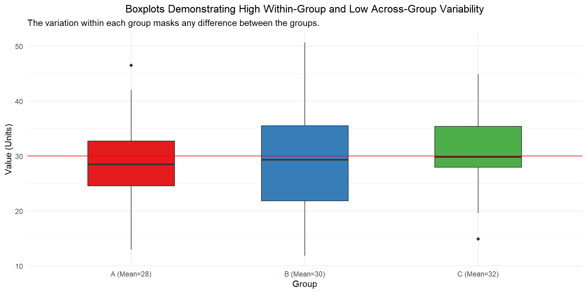
ANOVA is an extension from difference in means, where the test statistic is the variability (variance) within group vs the variability (variance) across groups.
Are any of the means different?
Which ones are different?
A conversation
There is (some) debate on if Anova is necessary to perform before using tukeyHSD to find which means are different.
Anova first
Logistic guardrail
Applying a global test first is pretty solid protection against the risk of (even inadvertently) uncovering spurious “significant” results from post-hoc data snooping.
It is known that a global ANOVA F test can detect a difference of means even in cases where no individual test of any of the pairs of means will yield a significant result. In other words, in some cases the data can reveal that the true means likely differ but it cannot identify with sufficient confidence which pairs of means differ.
Example
              Df Sum Sq Mean Sq F value Pr(>F)
factor(group)  2 11.132   5.566    11.3 0.0401 *
Residuals      3  1.478   0.493
---
Signif. codes:  0 '***' 0.001 '**' 0.01 '*' 0.05 '.' 0.1 ' ' 1
Tukey multiple comparisons of means
95% family-wise confidence level
Fit: aov(formula = y ~ factor(group))
$`factor(group)`
diff lwr upr p adj
2-1 2.90306081 -0.03000355 5.836125 0.0513476
3-1 2.87565627 -0.05740809 5.808721 0.0526193
3-2 -0.02740454 -2.96046891 2.905660 0.9991602Anova
Example
Plants
What would our null and alternative hypotheses in words / notation be?
Plants
Ho: \(\mu_c = \mu_1 = \mu_2\)
Ha: at least one population mean weight across the three groups is different
Assumptions
– Independence
– Normality
– Equal Variance
Independence
– between groups
– across groups
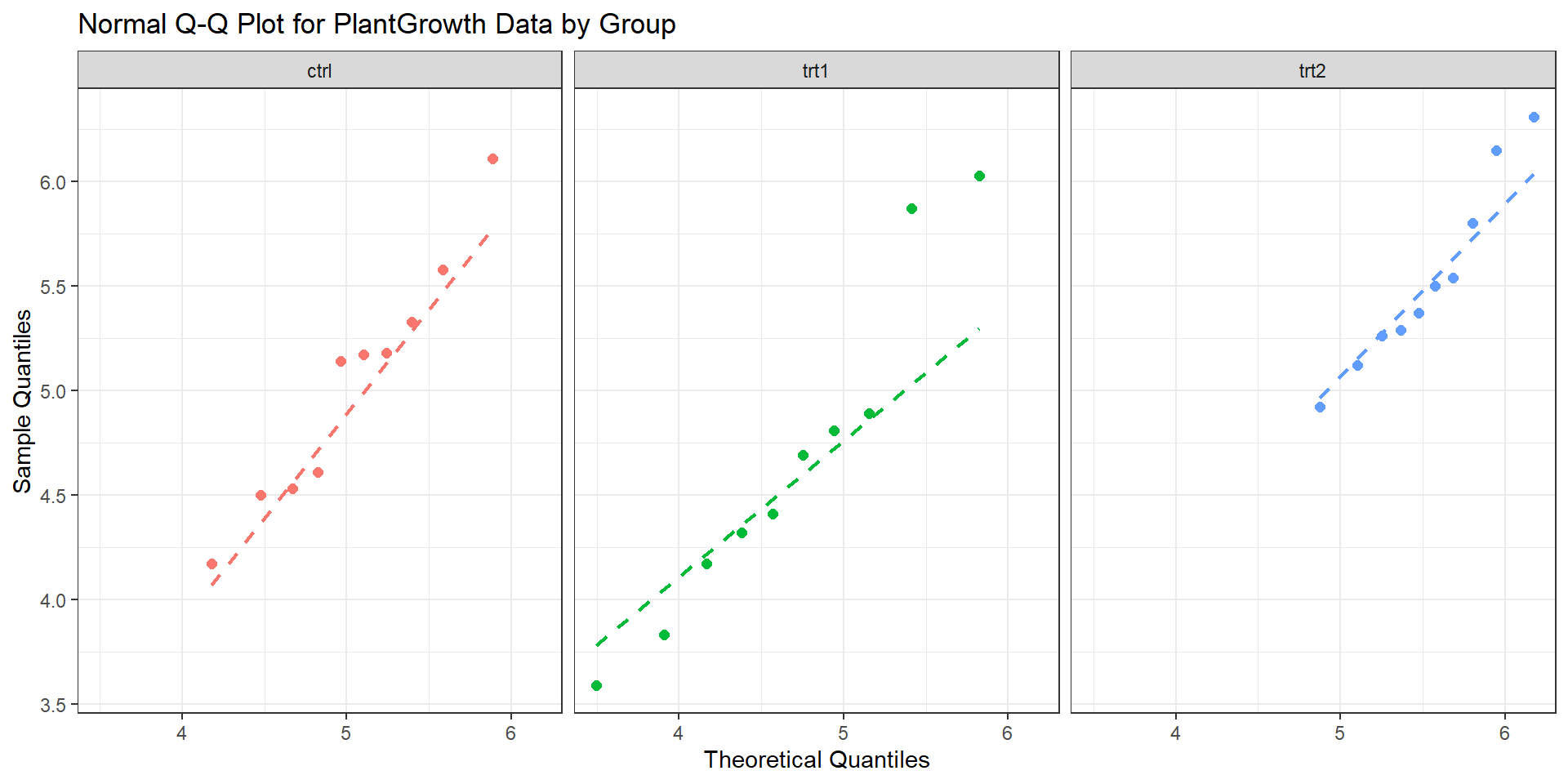
Normality
Plants q-q
Equal variance
# A tibble: 3 × 2
  group    sd
  <fct> <dbl>
1 ctrl  0.583
2 trt1  0.794
3 trt2  0.443
General rule: Is the largest sample standard deviation more than twice the smallest sample standard deviation?
New statistic
\(F = \frac{\text{MS}_{\text{Between}}}{\text{MS}_{\text{Within}}}\)
\(\mathbf{F} = \frac{\frac{\text{SS}_{\text{Between}}}{k - 1}}{\frac{\text{SS}_{\text{Within}}}{N - k}}\)
\(\text{SS}_{\text{Between}} = \sum_{i=1}^{k} n_i (\bar{X}_i - \bar{X}_{\text{grand}})^2\)
\(\text{SS}_{\text{Within}} = \sum_{i=1}^{k} \sum_{j=1}^{n_i} (X_{ij} - \bar{X}_i)^2\)
Draw it out
What would this look like?
That is, draw out how each SS would be calculated.
Plants
New statistic
\(F = \frac{\text{MS}_{\text{Between}}}{\text{MS}_{\text{Within}}}\)
\(\mathbf{F} = \frac{\frac{\text{SS}_{\text{Between}}}{k - 1}}{\frac{\text{SS}_{\text{Within}}}{N - k}}\)
\(\text{SS}_{\text{Between}} = \sum_{i=1}^{k} n_i (\bar{X}_i - \bar{X}_{\text{grand}})^2\)
\(\text{SS}_{\text{Within}} = \sum_{i=1}^{k} \sum_{j=1}^{n_i} (X_{ij} - \bar{X}_i)^2\)
Definitions
The Sum of Squares (SS) is a measure of total variability (between or within)
The Mean Squares (MS) is an estimate (\(s^2\)) of the population variance (\(\sigma^2\))
It’s a generalized form of \(s^2 = \frac{\sum(x_i - \bar{x})^2}{n-1}\)
Deviations divided by degrees of freedom!
Anova
Df Sum Sq Mean Sq F value Pr(>F)
group 2 3.766 1.8832 4.846 0.0159 *
Residuals 27 10.492 0.3886
---
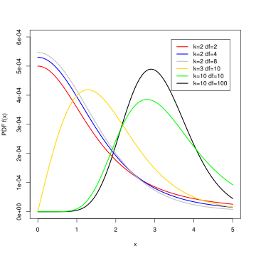
Signif. codes: 0 '***' 0.001 '**' 0.01 '*' 0.05 '.' 0.1 ' ' 1F-distribution
A continuous, positively skewed probability distribution, characterized by two degrees of freedom (numerator and denominator) that determine its shape.
Anova
Where did all of this come from?
The goal is not for you to be able to calculate these values by hand (besides Df). The goal is for you to understand the relationships between the values of the Anova table.
            Df Sum Sq Mean Sq F value Pr(>F)
group        2  3.766  1.8832   4.846 0.0159 *
Residuals   27 10.492  0.3886
---
Signif. codes:  0 '***' 0.001 '**' 0.01 '*' 0.05 '.' 0.1 ' ' 1
Anova table
Where did we get df = 2 for between? Where did we get df = 27 for within?
# A tibble: 3 × 2
  group     n
  <fct> <int>
1 ctrl     10
2 trt1     10
3 trt2     10
degrees of freedom
Degrees of Freedom (df) is the number of independent pieces of information used to calculate the statistic
When we estimate the population (grand) mean, there are k-1 independent pieces of information
When we estimate the population means within each group, there are n - k independent pieces of information
Anova: MS
The Mean Squares (MS) is an estimate (\(s^2\)) of the population variance (\(\sigma^2\))
It’s a generalized form of \(s^2 = \frac{\sum(x_i - \bar{x})^2}{n-1}\)
In Anova, it’s calculated by taking \(\frac{SS}{df}\)
            Df Sum Sq Mean Sq F value Pr(>F)
group        2  3.766  1.8832   4.846 0.0159 *
Residuals   27 10.492  0.3886
---
Signif. codes:  0 '***' 0.001 '**' 0.01 '*' 0.05 '.' 0.1 ' ' 1
Anova: F-statistic
The whole goal of Anova is to compare the variability between groups vs the variability within groups. How can we calculate our F-statistic?
            Df Sum Sq Mean Sq F value Pr(>F)
group        2  3.766  1.8832   4.846 0.0159 *
Residuals   27 10.492  0.3886
---
Signif. codes:  0 '***' 0.001 '**' 0.01 '*' 0.05 '.' 0.1 ' ' 1
Decision and conclusions
What are they? At the \(\alpha\) = 0.05 level.
So what’s actually different?
Which one(s)?
Tukeys HSD
The main idea of the hsd is to compute the honestly significant difference (hsd) between all pairwise comparisons
Why do we need to use this thing called Tukeys hsd? Why can’t we just conduct a bunch of individual hypothesis tests?
Type 1 error
\(\alpha\) is our significance level. It’s also our Type 1 error rate.
a Type 1 error is:
– rejecting the null hypothesis
– when the null hypothesis is actually true
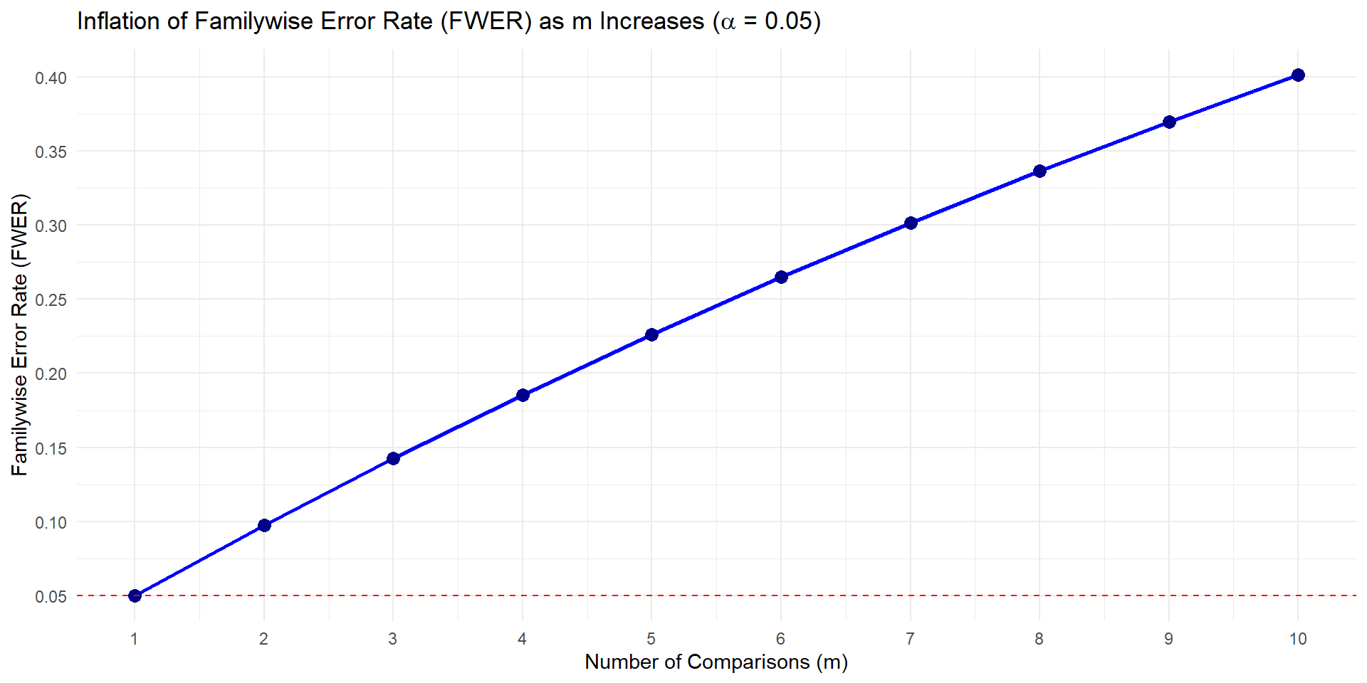
Family-wise error rate
FWER = \(1 - (1-\alpha)^m\)
where m is the number of comparisons
Family-wise error rate
Chocolate study

Learning objectives
– Why we use tukeysHSD
– What distribution we use to account for the inflated type-1 error rate
– How we do this in R
– How to read R output
Pairwise comparisons
Commonly report confidence intervals to estimate which means are actually different (also reports p-values).
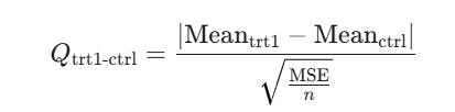
tukey’s hsd (technically Tukey-Kramer with unequal sample size)
\(\bar{x_1} - \bar{x_2} \pm \frac{q^*}{\sqrt{2}}* \sqrt{MSE*\frac{1}{n_j} + \frac{1}{n_j`}}\)
Where
– \(q^*\) is a value from the studentized range distribution
– (MSE) refers to the average of the squared differences between individual data points within each group and their respective group mean
\(q^*\) can be found using the qtukey function, or here
We are going to use a pre-packaged function in R to do the above calculations for us.
Results
Summary
Tukey’s Honest Significant Difference (HSD) test is a post hoc test commonly used to assess the significance of differences between pairs of group means. Tukey HSD is often a follow up to one-way ANOVA, when the F-test has revealed the existence of a significant difference between some of the tested groups.