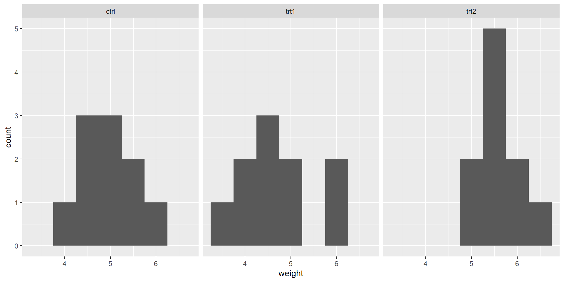
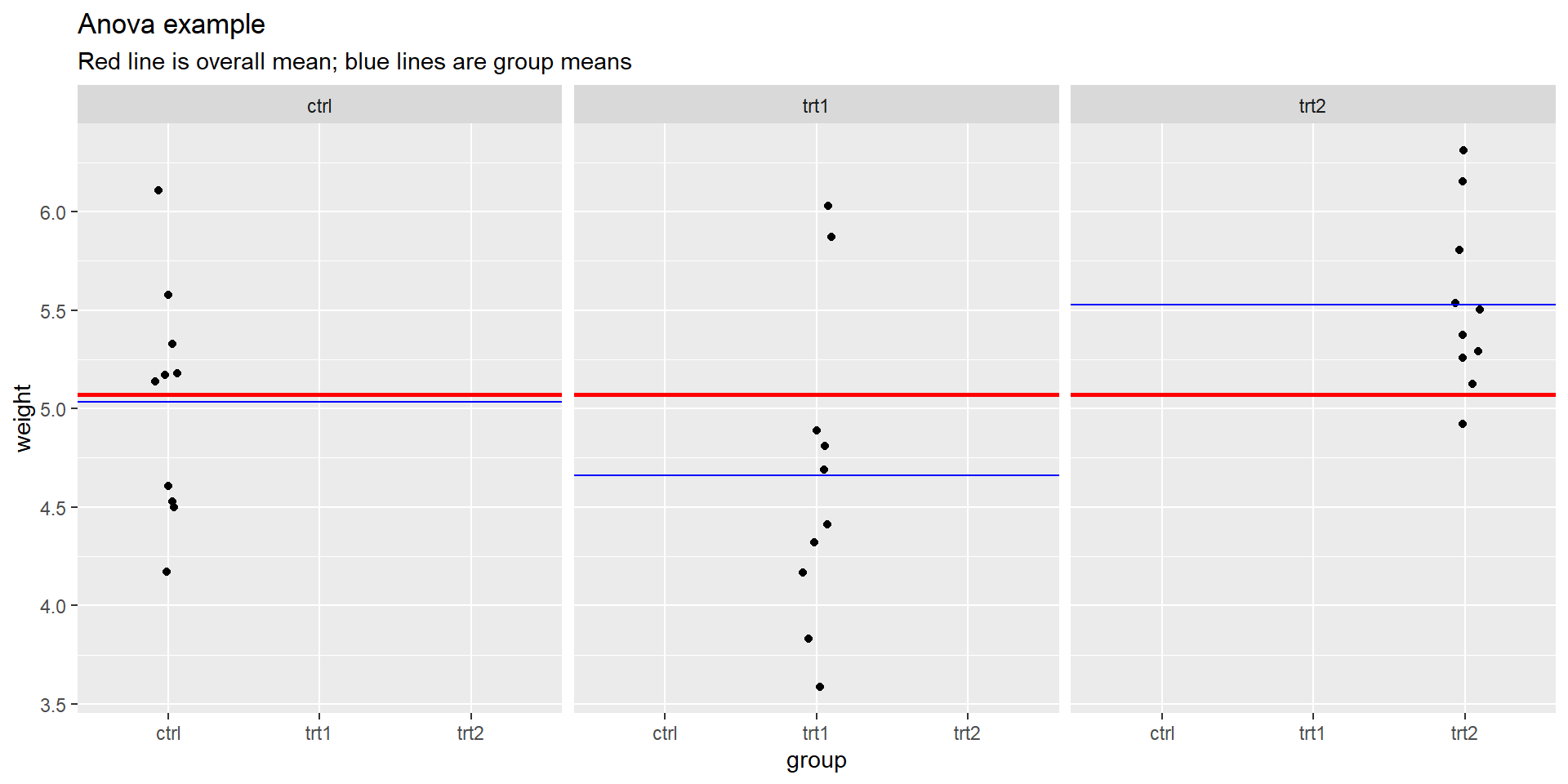
# A tibble: 3 × 3
group count mean
<fct> <int> <dbl>
1 ctrl 10 5.03
2 trt1 10 4.66
3 trt2 10 5.53One-way Anova
Dr. Elijah Meyer
NC State University
ST 511 - Fall 2025
2025-10-15
Checklist
– Takehome exam is due Friday at 11:59pm
  > Please do not wait until the last minute
  > There is no late policy on the takehome
– In-class exams are (almost) graded
> My goal is by Friday
– Next exam is the final exam
> There will not be a takehome component
– No homework this week
– No quiz this week
– Thursday October 23rd is the drop/revision deadline for Fall semester.
Hypothesis Testing Review
We are going to talk through the broad steps / ideas to make sure we have a firm understanding of the concepts
Questions
New context

Results from an experiment to compare yields (as measured by dried weight of plants) obtained under a control and two different treatment conditions.
Why can we not answer this question using difference in means?
Extension
ANOVA is an extension from difference in means, where the test statistic is the variability (variance) within group vs the variability (variance) across groups.
Example
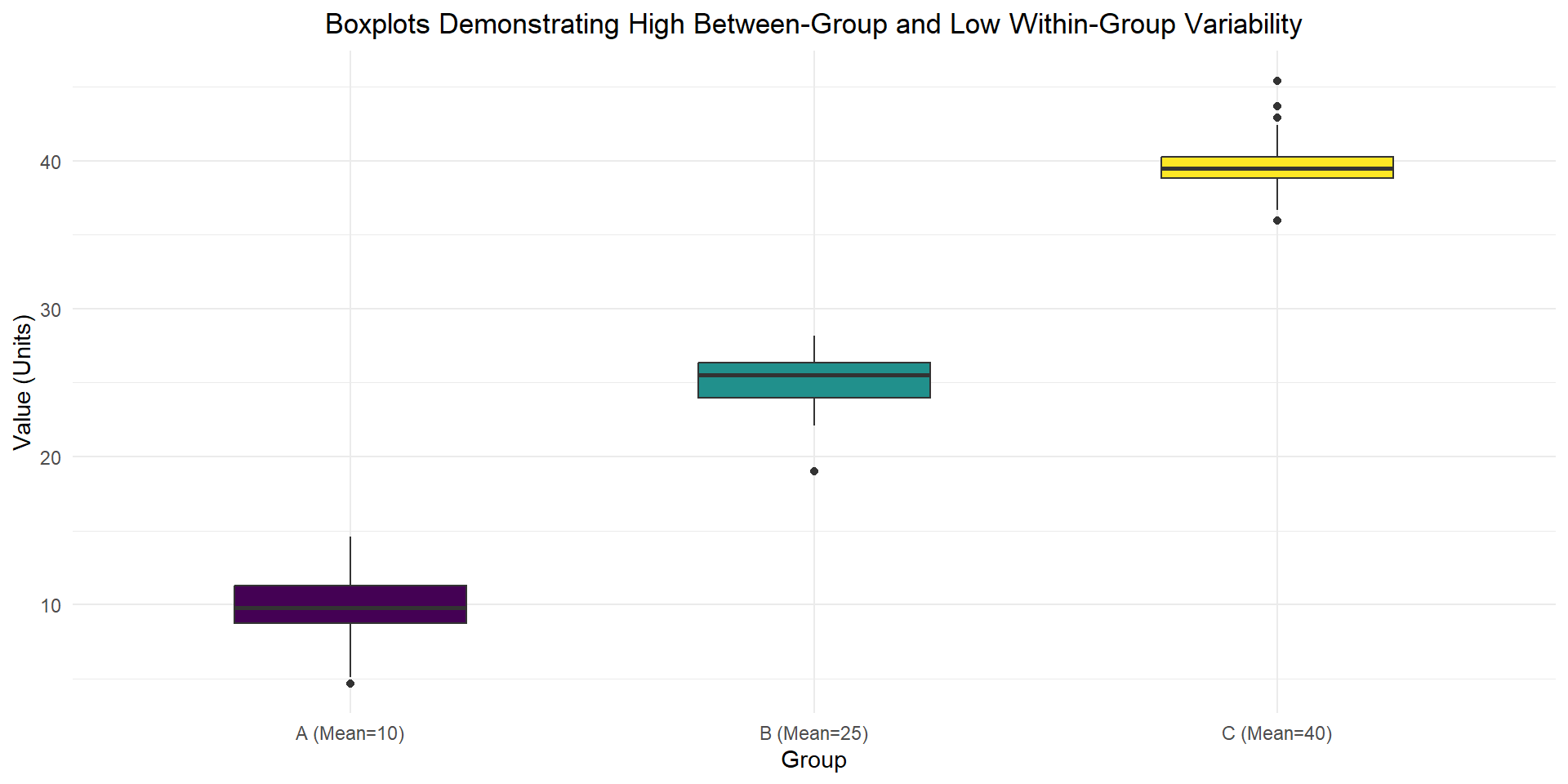
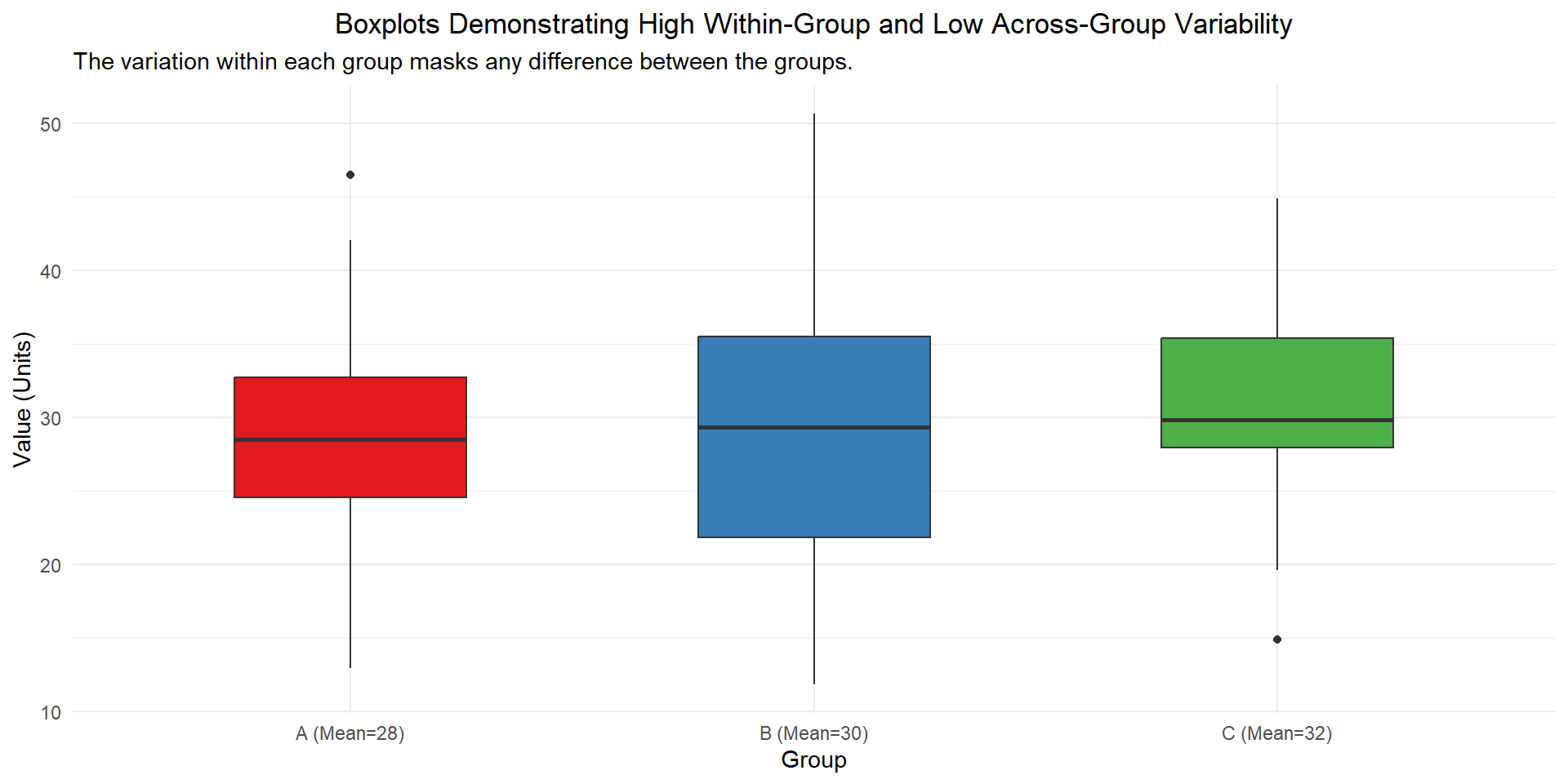
Plants
What would our null and alternative hypotheses in words / notation be?
Plants
Ho: \(\mu_c = \mu_1 = \mu_2\)
Ha: at least one population mean weight across the three groups is different
Assumptions
– Independence
– Normality
– Equal Variance
Independence
– between groups
– across groups
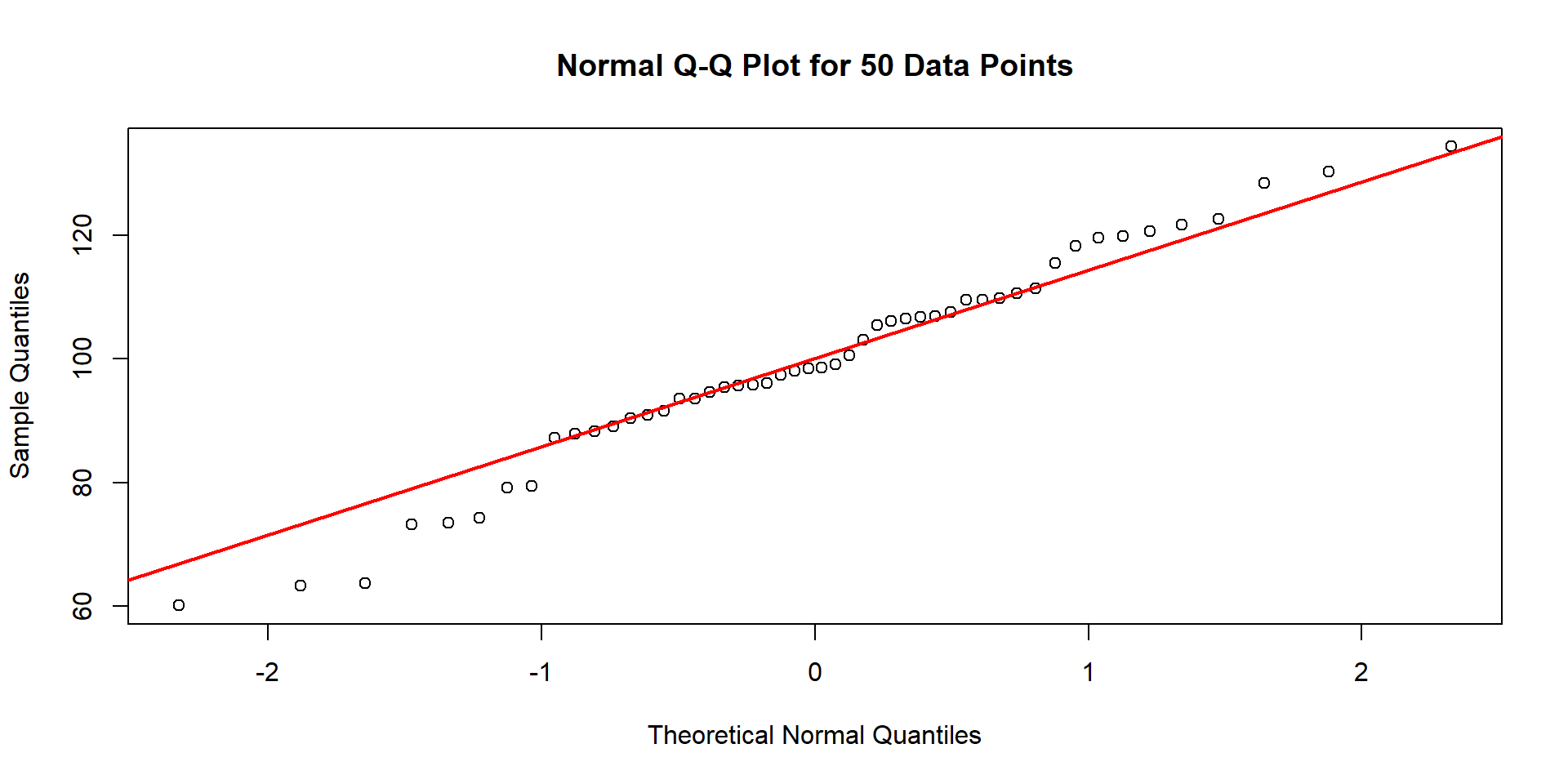
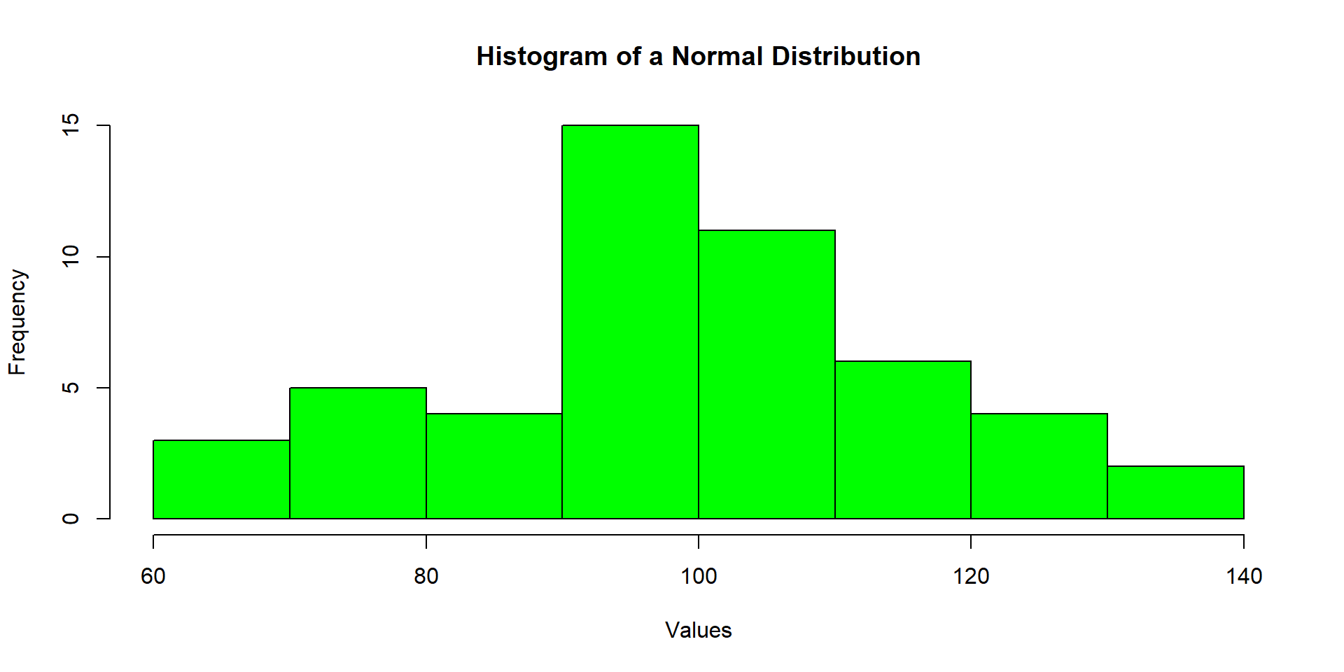
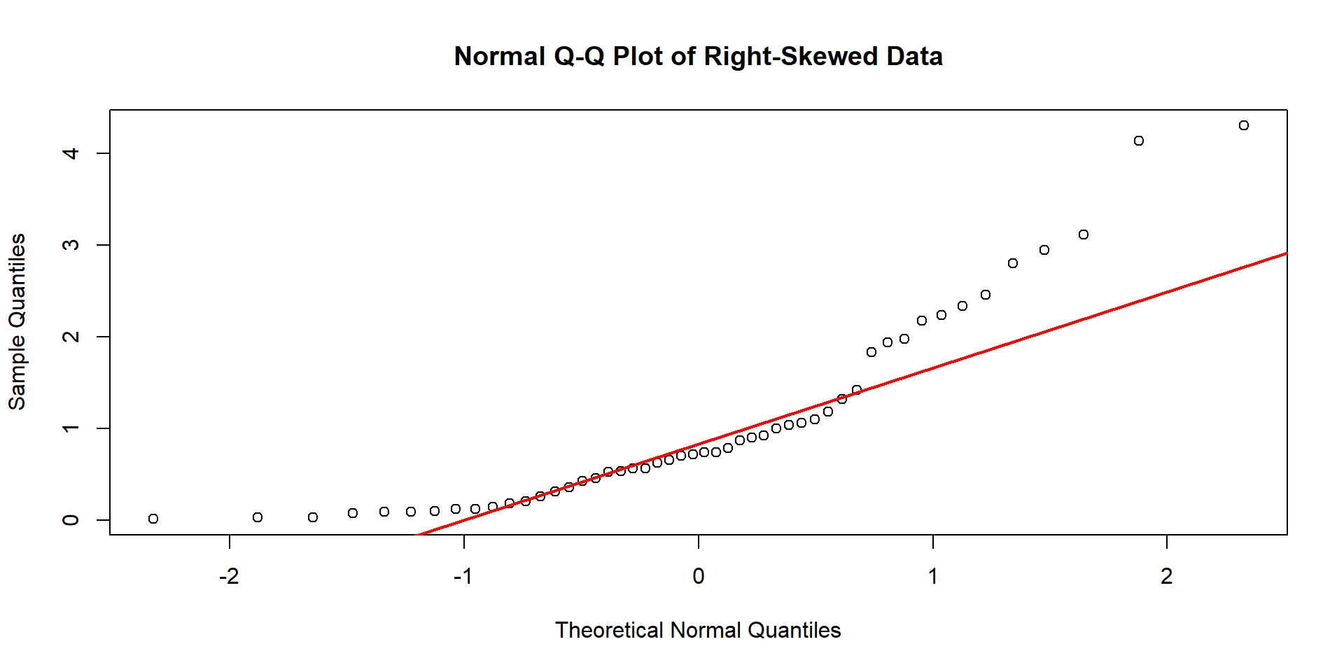
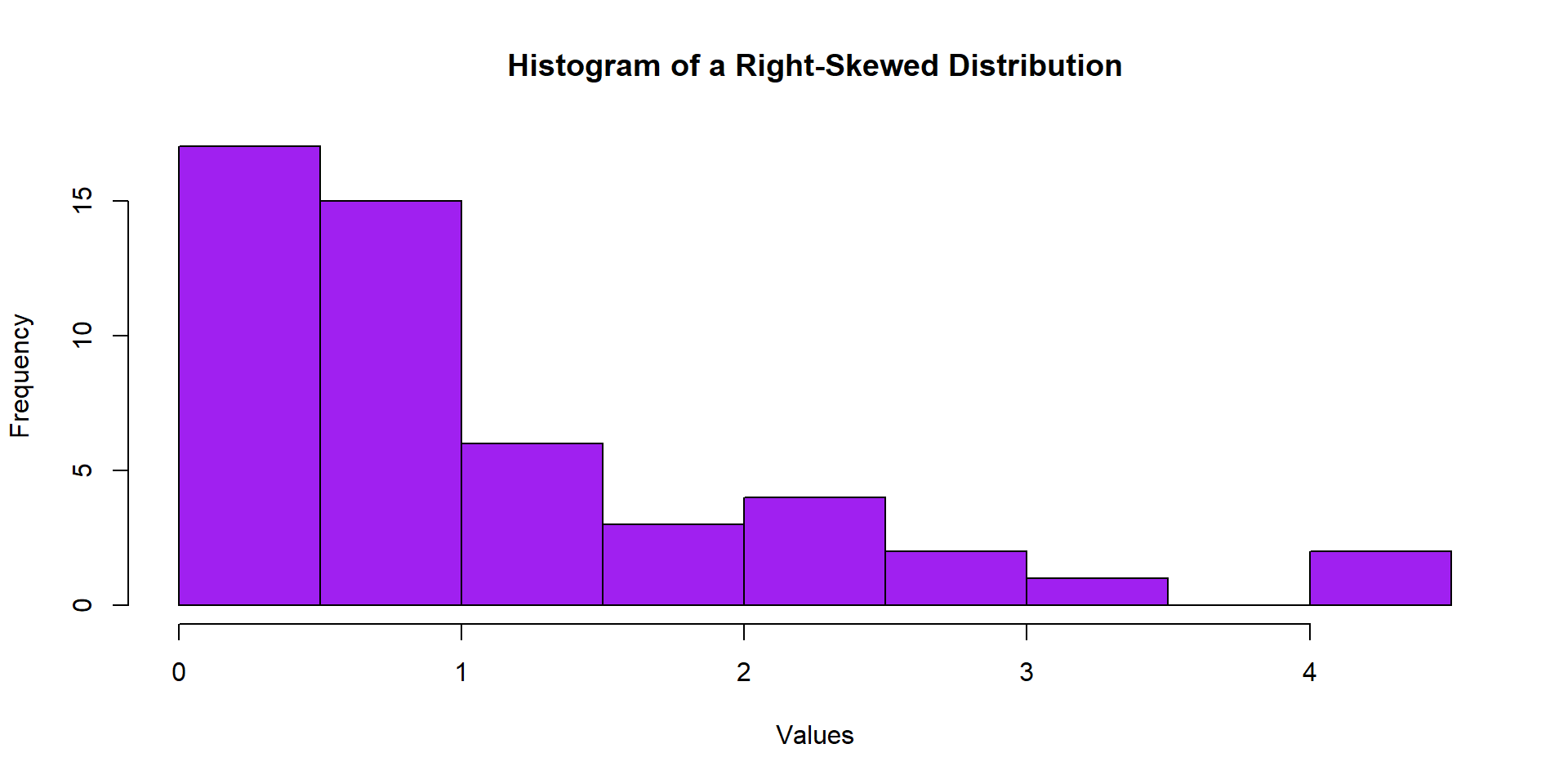
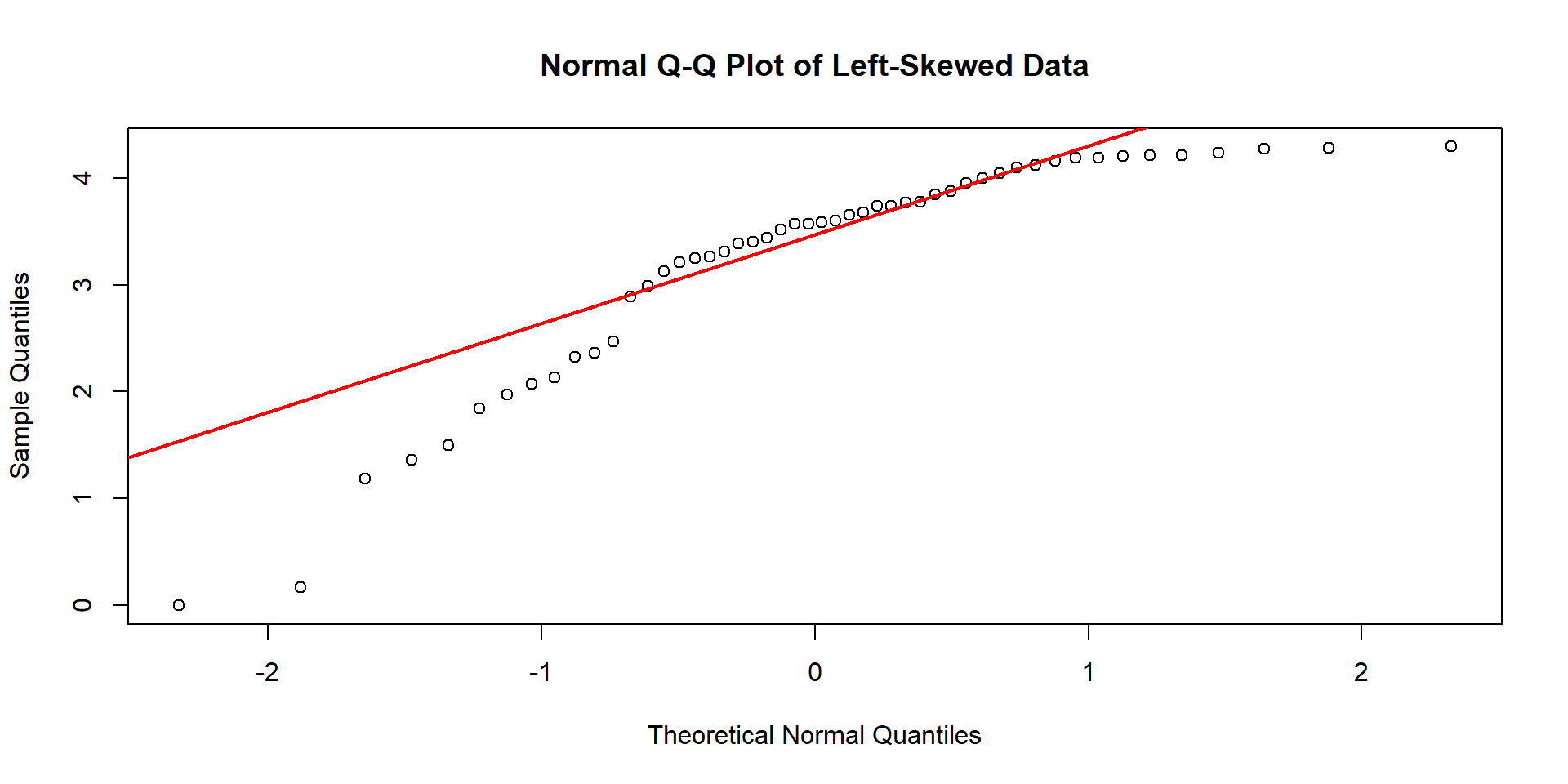
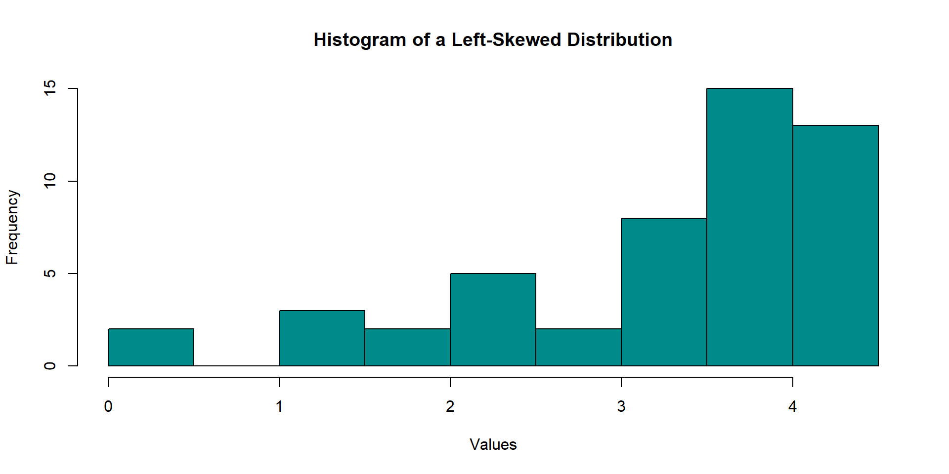
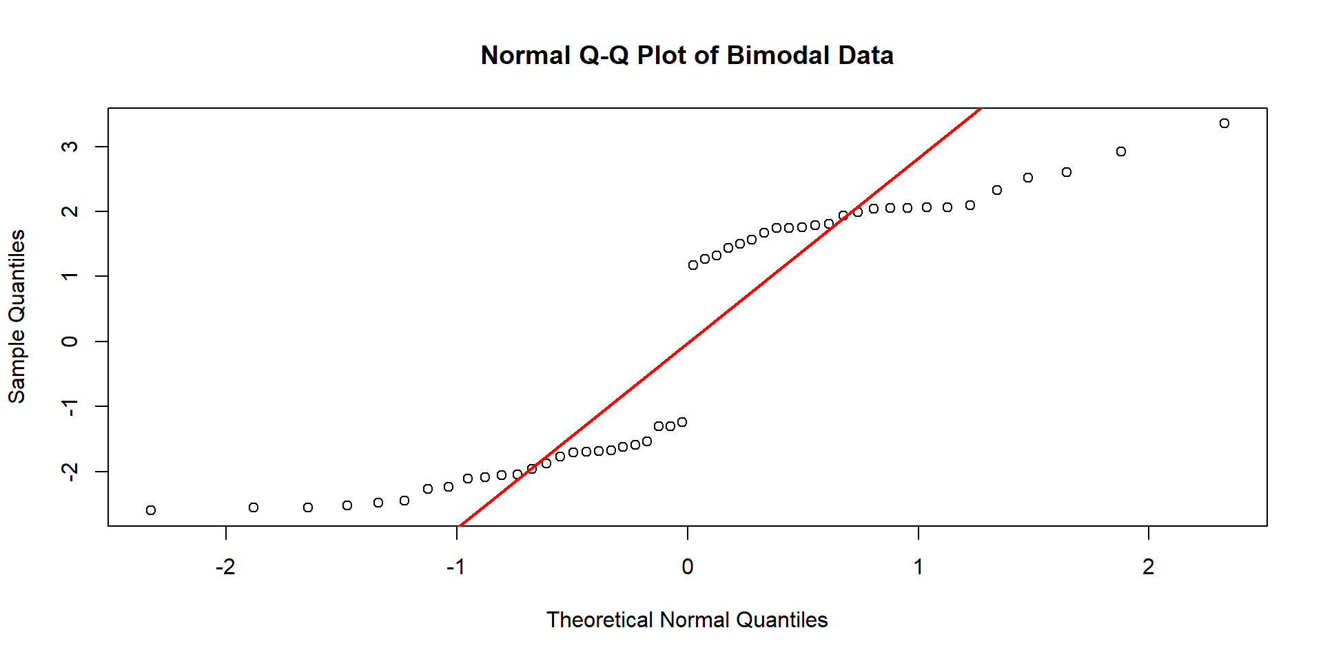
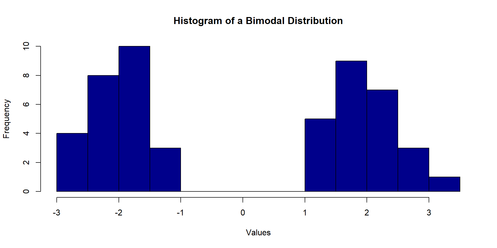
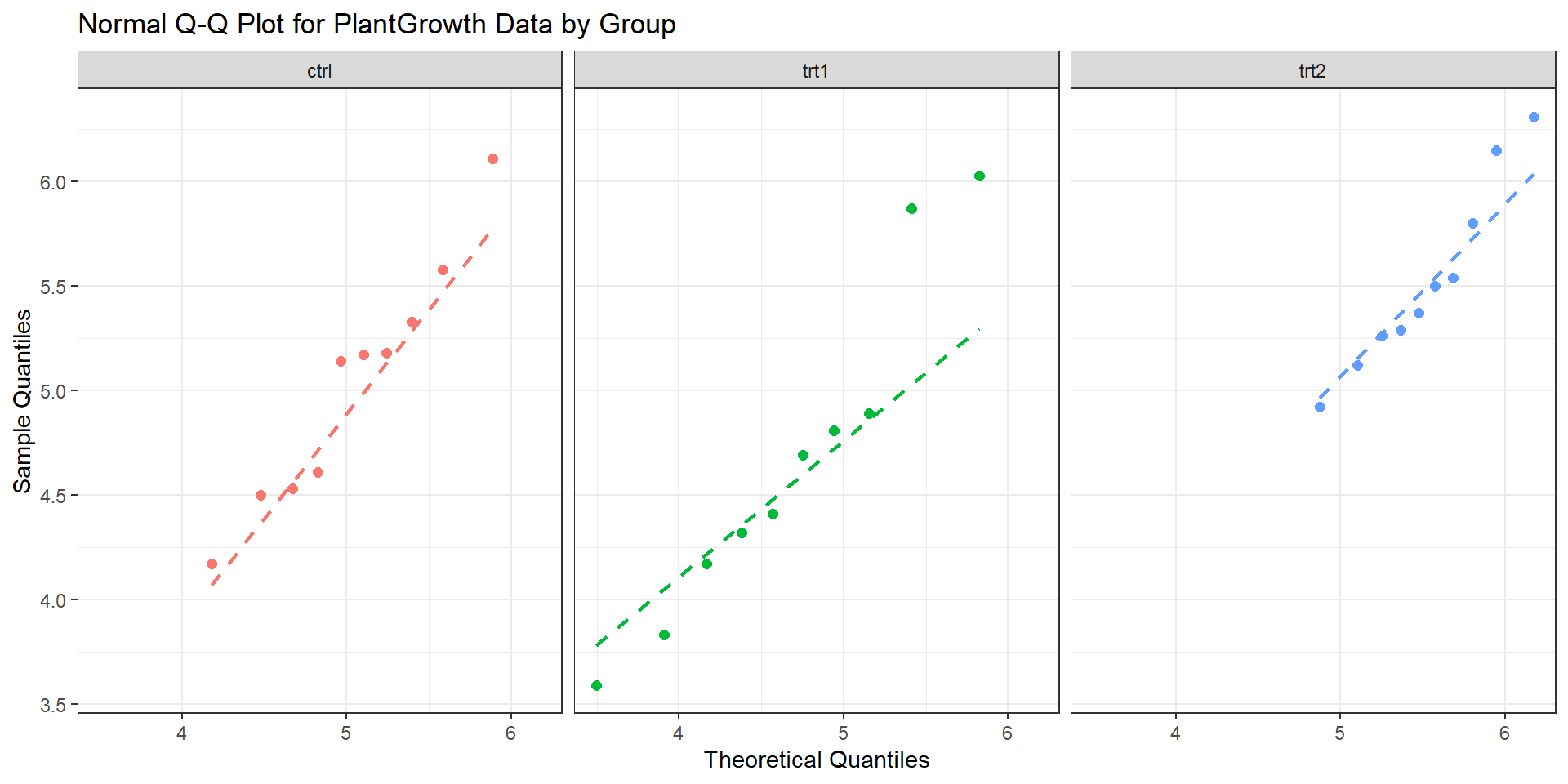
Normality
Normality
But sometimes, it is hard to tell just from the plot alone…
So we can use quantiles and a Normal q-q plot to help us better understand if our data appear normally distributed.
In short: We plot the values we observe from our data set versus what we would expect our values to be if they truely followed a normal distribution.
– If the dots mostly follow a straight line, we have evidence of normality!
– If they do not… we have evidence of skew
different looking q-q plots
Questions?
Our context
Normal q-q video
Equal variance
# A tibble: 3 × 2
  group    sd
  <fct> <dbl>
1 ctrl  0.583
2 trt1  0.794
3 trt2  0.443
General rule: Is the largest sample standard deviation more than twice the smallest sample standard deviation?
New statistic
\(F = \frac{\text{MS}_{\text{Between}}}{\text{MS}_{\text{Within}}}\)
\(\mathbf{F} = \frac{\frac{\text{SS}_{\text{Between}}}{k - 1}}{\frac{\text{SS}_{\text{Within}}}{N - k}}\)
\(\text{SS}_{\text{Between}} = \sum_{i=1}^{k} n_i (\bar{X}_i - \bar{X}_{\text{grand}})^2\)
\(\text{SS}_{\text{Within}} = \sum_{i=1}^{k} \sum_{j=1}^{n_i} (X_{ij} - \bar{X}_i)^2\)
Draw it out
What would this look like?
That is, draw out how each SS would be calculated.
Plants
Anova
F-distribution
A continuous, positively skewed probability distribution, characterized by two degrees of freedom (numerator and denominator) that determine its shape.
Anova
Where did all of this come from?
The goal is not for you to be able to calucalte these values by hand (besides Df). The goal is for you to understand the relationships between the values of the Anova table.
            Df Sum Sq Mean Sq F value Pr(>F)
group        2  3.766  1.8832   4.846 0.0159 *
Residuals   27 10.492  0.3886
---
Signif. codes:  0 '***' 0.001 '**' 0.01 '*' 0.05 '.' 0.1 ' ' 1
Definitions
Degrees of Freedom (df) is the number of independent pieces of information used to calculate the statistic
The Sum of Squares (SS) is a measure of total variability (between or within)
The Mean Squares (MS) is an estimate (\(s^2\)) of the population variance (\(\sigma^2\))
It’s a generalized form of \(s^2 = \frac{\sum(x_i - \bar{x})^2}{n-1}\)
Anova table
Where did we get df = 2 for between? Where did we get df = 27 for within?
# A tibble: 3 × 2
  group     n
  <fct> <int>
1 ctrl     10
2 trt1     10
3 trt2     10
Anova: MS
The Mean Squares (MS) is an estimate (\(s^2\)) of the population variance (\(\sigma^2\))
It’s a generalized form of \(s^2 = \frac{\sum(x_i - \bar{x})^2}{n-1}\)
In Anova, it’s calculaed by taking \(\frac{SS}{df}\)
            Df Sum Sq Mean Sq F value Pr(>F)
group        2  3.766  1.8832   4.846 0.0159 *
Residuals   27 10.492  0.3886
---
Signif. codes:  0 '***' 0.001 '**' 0.01 '*' 0.05 '.' 0.1 ' ' 1
Anova: F-statistic
The whole goal of Anova is to compare the variability between groups vs the variability within groups. How can we calculate our F-statistic?
            Df Sum Sq Mean Sq F value Pr(>F)
group        2  3.766  1.8832   4.846 0.0159 *
Residuals   27 10.492  0.3886
---
Signif. codes:  0 '***' 0.001 '**' 0.01 '*' 0.05 '.' 0.1 ' ' 1
Decision and conclusions
What are they? At the \(\alpha\) = 0.05 level.
So what’s actually different?
Next time!