> your repo is called homework-2
> we will look at the number of commits you have
– Quiz released Wednesday (due Sunday at 11:59pm)
– Please clone the one-prop-test repo for today
– I wrote up a resource on random variables / probability distributions on our website! Check it out.
Goals for today
– Carry out a hypothesis test for single proportion
– Introduce the idea of confidence intervals
Warm-up
Click-through rate (CRT) is the proportion of users that click on a specific add. Using the context below, set up the null and alternative hypothesis. Also write out the sample statistic in proper notation.
A company has historically seen a 12% click-through rate (CTR) on its banner ads. The marketing team launches a new, redesigned ad and wants to know if it’s more effective. They run the new ad and collect data from a random sample of 1,500 potential customers. In this sample, 210 people clicked on the ad.
Warm-up
\(Ho: \pi = .12\)
\(Ha: \pi > .12\)
\(\hat{p}\) = \(\frac{210}{1500}\)
Warm-up
Using the context below, set up the null and alternative hypothesis. Also write out the sample statistic in proper notation.
A lightbulb manufacturer claims that its new LED lightbulb has an average lifespan of 1,000 hours. A consumer advocacy group wants to test this claim. They purchase a random sample of 30 lightbulbs and test them, finding the average lifespan of their sample is 985 hours.
Warm-up
\(Ho: \mu = 1000\)
\(Ha: \mu \neq 1000\)
\(\bar{x} = 985\)
What is Hypothesis Testing
– We make an assumption
– We collect data
– We see how unlikely it is to observe that data if our assumption is true!
… and we know sampling variability exists… we we compare our sampled data vs a sampling distribution!
one-prop-test AE
LaTeX Code
\(\mu\) = $mu$
\(\pi\) = $pi$
\(\hat{p}\) = $hat{p}$
\(H_o\) = $H_o$
We have a demo on our website for more information!
The list goes on….
LaTeX Code
LaTeX is not a requirement for this course. If you want the opportunity to build up this skill, please do so.
\(\mu\) = mu
\(\pi\) = pi
\(\hat{p}\) = p-hat
\(H_o\) = Ho
The list goes on….
Bumba vs Kiki
Hypothesis Testing
Set up a null and alternative hypothesis
Collect data
Check assumptions
Analyze data
Make decisions and conclusions
Assumptions
For our hypothesis test, we need to check the following assumptions:
– Independence (do we satisfy this condition?)
– Normality
Normality
\(\pi_o\) = \(p_o\)
– n* \(\pi_o\) > 10
– n* (1 - \(\pi_o\)) > 10
Do we satisfy this condition?
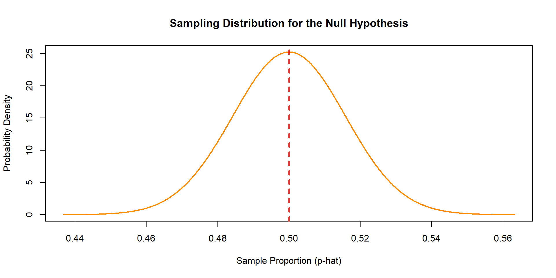
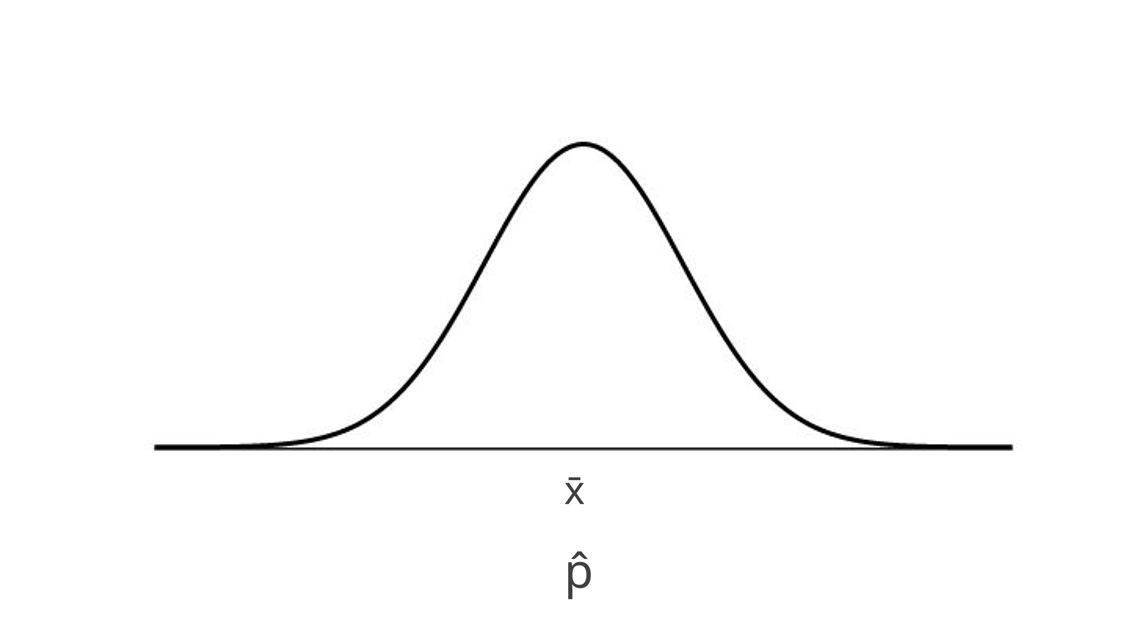
Sampling Distribution of p-hat
Centered at the null value will look like….
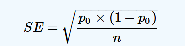
What is the standard error of the sampling distribution?
Note: The standard deviation of the sampling distribution is called the standard error!
Quantifies how much you can expect the statistic from any sample to vary from the true population parameter (center)
p-value
What is it? How do we calculate it?
Replace test_stat, null_mean, ect with the appropriate values
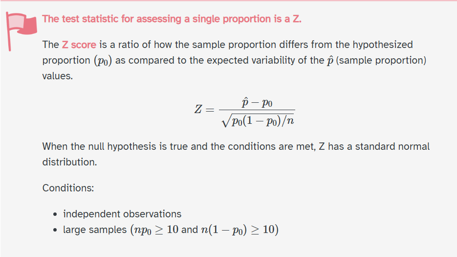
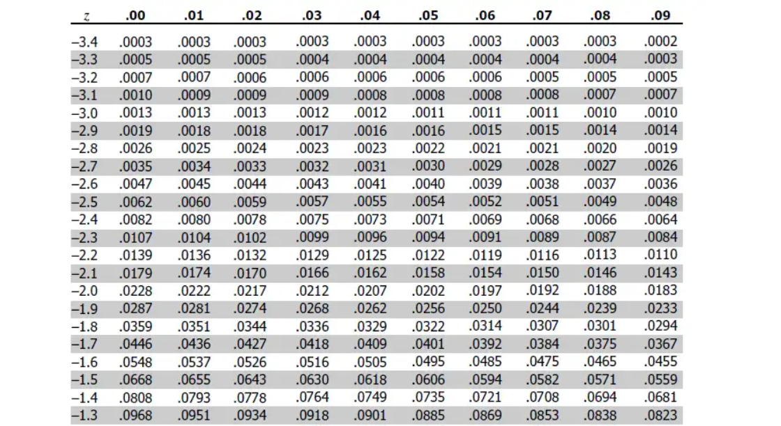
Z-distribution
Standardized Statistic
Why?
Before technology, a bunch of people did some really hard calculus, so the probabilities of a standard normal distribution were known.
Standardized Statistic
Why today?
– It helps us compare Z-scores across studies (has no units)
– It’s a common practice most fields still use
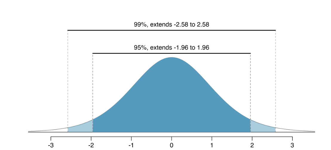
Confidence Intervals
Hypothesis Tests are great when we want to garner evidence if our population parameter is larger, smaller, or different than some value.
Confidence intervals allow us to estimate the population paramter we are interested in!
Motivation
What’s the true average battery life for a Google Pixel 9 cell phone?
Guesses?
Do you feel good about your guess?
Motivation
Suppose you took a random sample of 40 phones and calculated \(\bar{x}\) to be 18.5 hours.
How comfortable do you feel saying \(\mu\) = 18.5?
Motivation
Suppose you took a random sample of 40 phones and calculated \(\bar{x}\) to be 18.5 hours.
How comfortable do you feel saying \(\mu\) = 18.5?
Well this is our best guess for what \(\mu\) could be…. but
not really confident….. because sampling variability exists!
Confidence Interval Goal
We want to create a sampling distribution around our statistic, and use the standard error (sampling variability) to provide a range of values to estimate our population parameter.
Howling Cow Example
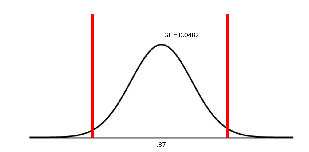
We want to estimate the number of NC State students that eat ice creme. Let’s assume that 100 NC State students were randomly sampled, and it turned out that \(\hat{p}\) = .37. This is our best guess for \(\pi\), which nobody thinks is actually correct.
Checking Assumptions
We need to make sure we understand how our sampling distribution will look, so we check assumptions!
– Independence (same as hypothesis testing)
– success-failure (sampling size); slightly different than hypothesis testing
success-failure
– Hypothesis testing: successes and failures under the assumption of the null hypothesis
– Confidence interval: successes and failures from our random sample
Howling Cow Assumption Check
– Independence
– Success Failure
\(\hat{p} = .37\)
n = 100
Howling Cow
Because our assumptions are satisfied, we know that our sampling distribution will be ~ Normal, and we can estimate the standard error of our sampling distribution as follows: