Foundations of Inference
Lecture 8
NC State University
ST 511 - Fall 2025
2025-09-10
Checklist
– HW-1 late window (11:59pm tonight on Gradescope)
– Quiz-3 released (due Sunday)
– HW-2 released Monday (due following Sunday)
– Our warm-up question will be in the finish-ggplot project from Monday
Last time
Does order matter?
Why did we spend time on data visualization?
– Every good data analysis starts with a good data exploration
– Effective data visualization when communicating to a larger audience
Why did we spend time on data visualization?
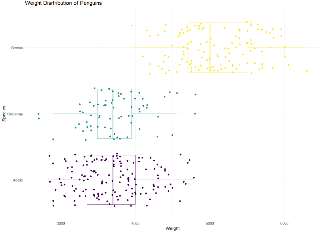
Impacts of professional development focused on teaching engineering applications of mathematics and science
Inference
Goals
– Understand common statistical terminology (population vs sample)
– Random variables
– Probability distributions
– Sampling distributions
– Central Limit Theorem
– Sampling schemes
Terms
Poupuatlion
Population level
Terms
– Population: The complete set of observational units you are collecting data on
Examples
– All NC State Students
– All fish in the Missouri river
– All trees in Umstead State Park
The Big Picture
– Want to make a claims about a population
– We need a way to quantify variability of a random variable so we can make claims about the population we are interested in
The process
Knowing the following concepts lays the foundation for us to perform inference
– Random Variables
– Probability distributions
– Sampling distributions
What’s a Random Variable?
Random Variables
Ways to map random process to numbers
What do we mean by a random process?
Random Variables
Random variables can be discrete or continuous
\[ X = \begin{cases} 1 & \text{if heads}\\ 0 & \text{if tails} \end{cases} \]
Random Variables
Random variables can be discrete or continuous
The height of a person. (A person’s height can be 5.9 feet, 5.91 feet, 5.912 feet, etc., within a certain range).
Example: The amount of rainfall in a day (can be measured in inches)
Why do we care?
Why do we care?
A random variable can take on many many values
This allows us to quantify the outcomes of random phenomena and apply statistical tools to analyze them
Why do we care?
Random variables are the building blocks of probability distributions
A probability distribution describes the set of all possible values a random variable can take and the probability of each value occurring
Probabilty distribution (discrete)
Your Turn
We flip a coin two times. The sample space is S = {HH, HT, TH, TT}. Let X be the number of heads.
Draw the probability distribution….
Probability distribution (cont)
In Practice
If we know the exact population distribution of a random variable, then we can use that to calculate probabilities!
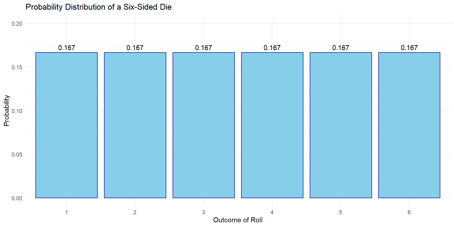
What’s the probability of rolling a 5 or a 6 on a 6-sided dice?
What’s the probability of rolling a 1 through 6?
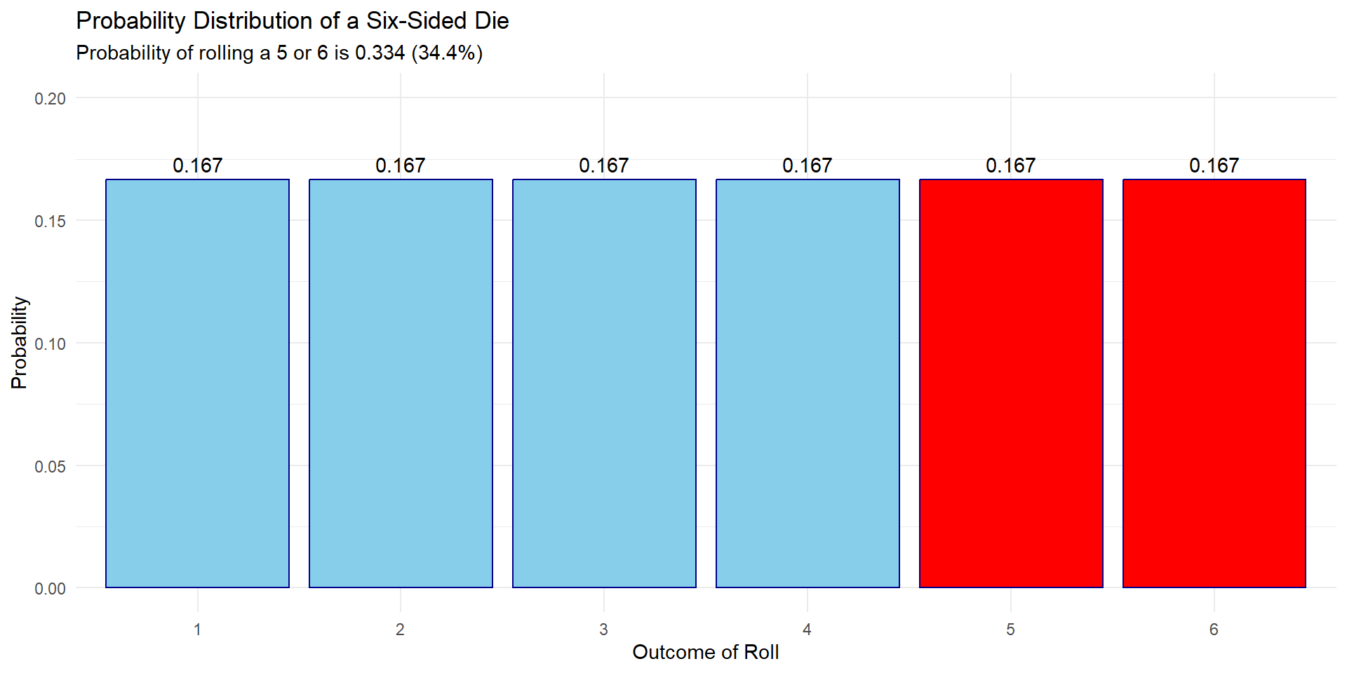
The area under the curve = 1
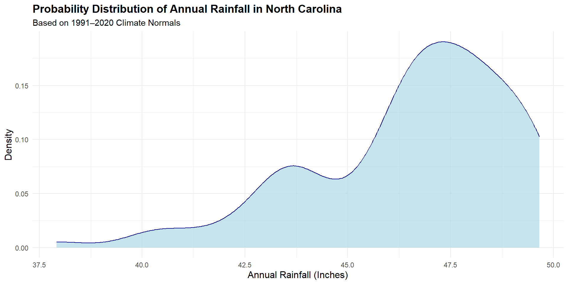
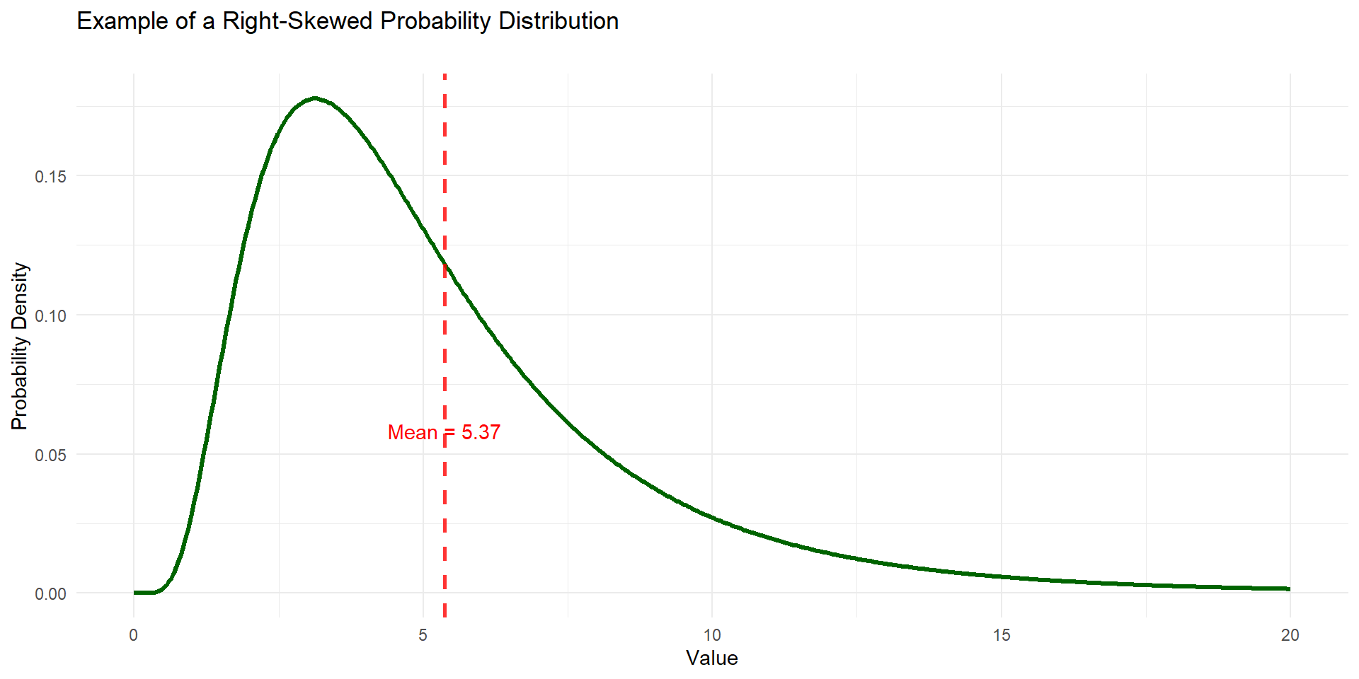
Example
What’s the probability that it rains more than 47.5 inches this year in NC?
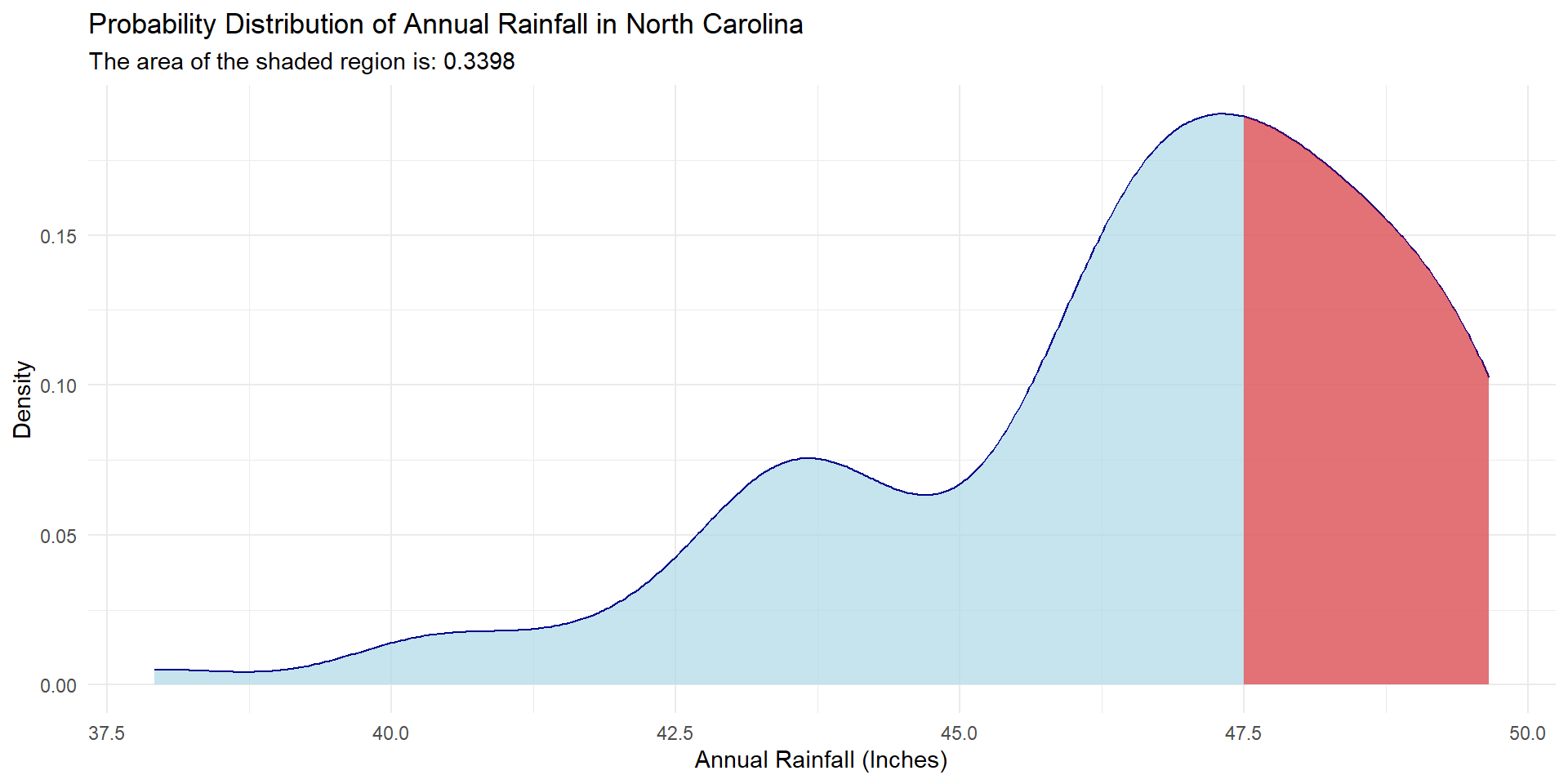
What’s the probability that it rains exactly 47.5 inches this year in NC?
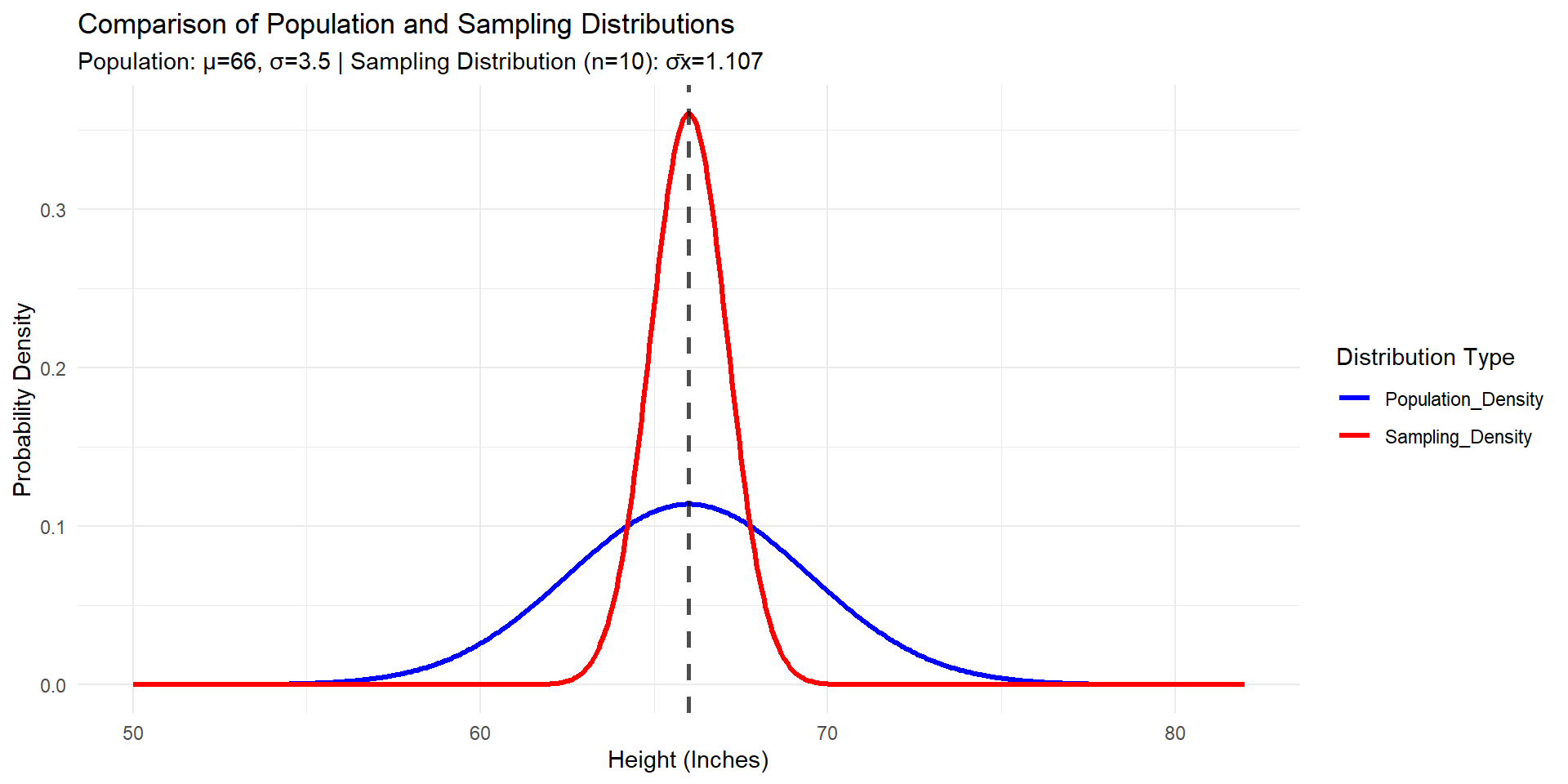
Probability and Sampling distribution
The probability distribution of a population directly influences the sampling distribution of a statistic drawn from that population. A sampling distribution is essentially the probability distribution of a statistic (like the sample mean or sample proportion) from all possible samples of a given size.
What do we mean by directly influence
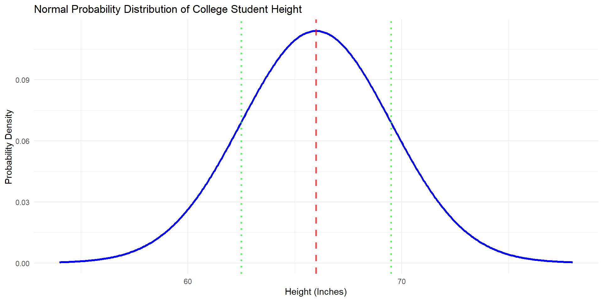
Normality
If the probability distribution is normal, the sampling distribution will be normal as well!
– z-tests
– t-tests
– Anova
…. and more run on the assumption of normality for the sampling distribution!
Pause
What do we mean by normal?
Describe what the following distributions look like:
– Normally distributed
– Right skewed
– Left skewed
– Bimodal
– Uniform
Example
Sampling distribution
Are the shapes different?
Are the centers different?
What if the population distribution is not normal?
Example
We are going to create a sampling distribution from this distribution to explore this idea!
n = 30
You save this as the object a using the assigmnet arrow and take the mean(a) to calculate the mean.
– Run the code
– Take the mean
– We are going to plot the means together and start to see what’s happening!
And if we kept going….

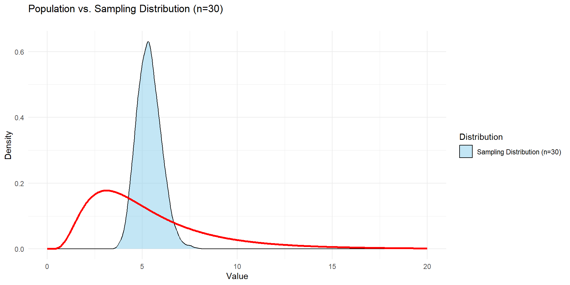
The Central Limit Theorem
For a large enough sample size (n > 30) and independent samples, regardless of what the population distribution looks like, the sampling distribution of the sample mean will be normally distributed with mean \(\mu\) and standard error of \(\frac{\sigma}{\sqrt(n)}\)
An assumption of z and t-tests is that the sampling distribution is normally distributed!
Note
This also works for proportions! We will talk more about this in detail when we start inference next week.
Demo in Stat Crunch
Let’s try it with the Uniform Distribution
Why this is so cool
When the data come from the random sample
– \(\bar{x}\) is an unbiased estimator for \(\mu\)
– The spread of the sampling distribution is \(\frac{\sigma}{\sqrt(n)}\)
Sampling
In practice, we typically only get a single sample, and assume that our \(\bar{x} \sim N(\mu, \frac{\sigma}{\sqrt{n}})\)
We estimate \(\mu\) with \(\bar{x}\) and we estimate \(\sigma\) with \(s\).
In practice
Sampling distributions are critical… here’s why…
Suppose I calculated the mean height of NC State students to be 64 inches (n = 10).
Should we then conclude that 64 inches is the population mean height of NC State students?
In practice
Can we conclude that 64 inches is significantly different than 67 inches?